Decision Tree – Halim Noor

Introduction

Decision tree is one of the most widely used machine learning algorithms in practice due to its being easy to understand and implement and more importantly, the output prediction is understandable. Decision tree is a non-parametric algorithm that can be used for both classification and regression problems [1]. The assumption of the decision tree algorithm is similar to k-nearest neighbors whereby data points are not randomly distributed in the feature space. Instead, data points belonging to a class tend to be close to each other, thus, appearing in clusters. K-nearest neighbors algorithm simply stores the training instances to perform predictions. Although the k-nearest neighbors algorithm is simple and can be powerful, it is memory intensive and computationally inefficient especially when the training set is large. Furthermore, what we are interested in is only the prediction. Consider a classification problem of YES and NO. If a test point falls in a cluster of YES, we will be able to immediately know that the test point belongs to YES before we calculate the distances. Therefore, the distance calculation is not really needed if the regions of YES and NO have been defined and we know in which region the test points fall.

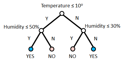
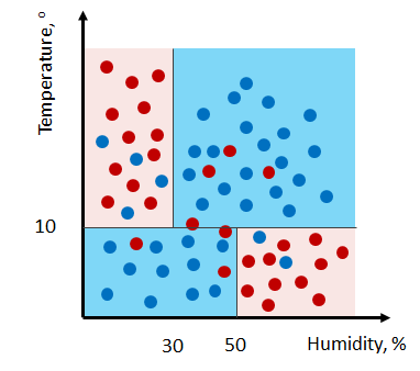
This idea is implemented in the decision tree algorithm. The decision tree algorithm does not store the training data. Instead, the training data is used to build a tree structure consisting of decision nodes and leaf nodes that divides that feature space into regions of similar labels. Consider a tree structure and its classification regions in Figure 1. The first node in the tree structure is the root node, which represents the whole training set which consists of two input features, Temperature, $x_1$ and Humidity, $x_2$ and two labels, YES and NO. This root node represents the first split whereby the training set is split along one dimension (Temperature) by defining a split-point or a threshold at $10^o$ . The split results in two sets of instances, one with all instances with $x_1 \leq 10^o$ and the others with $x_2$ at $50\%$ . Then, the region $x_1 \leq 10^o$ is split along $x_2$ at $50\%$ and the region $x_1 > 10^o$ is split along $x_2$ at $30\%$ . The decision tree has three decision nodes including the root node, which represent the condition for each feature split. The result of this process produces two regions representing the two labels indicated by the last four nodes known as the leaf nodes. Thus, in decision tree, we just need to store the conditions of the split and the labels. Given a test point, a decision tree performs the prediction by evaluating the test point against the condition of each nodes and traversing through the true branches until it reaches a leaf node. For example, given a test input $\mathbf{x}=(45,15)$ . The condition of the root node is false ( $x_2>10$ ). Thus we take the right branch and the following condition is false ( $x_1 > 30$ ). The right branch is taken and the input is predicted as YES.

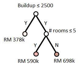
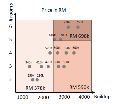
Figure 1. Decision tree and the classification regions.

Decision tree algorithm can be used for regression problems. Since the predicted value is a numerical value, the leaf nodes represent the mean of the responses of the instances in the regions. Consider a tree structure and its regression regions in Figure 2. The predicted values are estimated by the mean of the responses in the regression regions.

Figure 2. Decision tree and its regression (estimated) values.

Building a Tree

The accuracy of the prediction depends on where the split-point is defined for each decision node. To find the optimal split, we measure the reduction in randomness or uncertainty after the feature is split. The reduction in randomness is known as information gain. The information gain of splitting the set or node $t$ along feature, $x_j$ at a split-point, $s$ is given as follows:

$G(t, x_j, s) = H(t) - (\frac{\lvert t_l \rvert}{\lvert t \rvert}H(t_l) + \frac{\lvert t_r \rvert}{\lvert t \rvert}H(t_r))$

where $t_l$ and $t_r$ are the nodes (sets) of the left region (branch) and right region (branch) respectively after splitting $t$ at split-point $s$ . $\frac{\lvert t_{\eta} \rvert}{\lvert t \rvert}$ is the fraction of instances in branch $t_{\eta}$ . $H(t_{\eta})$ is the impurity function which measures quality of split or the homogeneity of the labels in set $t_{\eta}$ .

Classification

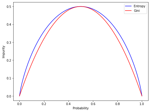
In the classification setting, there are two commonly used impurity functions which are entropy and gini. Entropy measures the uncertainty of the feature set. Entropy function is defined as follows:

$H(t)=-\sum_{c=1}^C p_c \log_2 p_c$

where $C$ is the number of class labels, $p_c$ is the probability of selecting an instance of class $c$ in node $t$ .

Gini measures the probability of a randomly chosen instance to be wrongly labeled. Gini function is defined as follows:

$H(t) = \sum_{c=1}^C p_c(1-p_c)=\sum_{c=1}^C p_c - \sum_{c=1}^C p_c^2 = 1-\sum_{c=1}^C p_c^2$

where $C$ is the number of class labels, $p_c$ is the probability of selecting an instance of class $c$ in node $t$ . For two classes, the node impurity is maximum when the subsets have an equal number of instances in which the probability of both classes is 0.5 as shown in Figure 3.

Figure 3. Impurity measures for binary classification. Entropy has been scaled to a range of [0,0.5].

Numerical Example

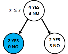
Consider the following split as shown in Figure 4. Calculate the entropy and gini measures and the information gain.

Information gain of the split with entropy measure

$H(t)=-(\frac{4}{7}\log_2\frac{4}{7} + \frac{3}{7}\log_2\frac{3}{7})=0.9852$

$H(t_l)=-(\frac{2}{2}\log_2\frac{2}{2} + \frac{0}{2}\log_2\frac{0}{2})=0.0$

$H(t_r)=-(\frac{2}{5}\log_2\frac{2}{5} + \frac{3}{5}\log_2\frac{3}{5})=0.9710$

$G(t,x_1,s)=0.9852 - \frac{2}{7}(0) - \frac{5}{7}(0.9710)=0.2916$

Information gain of the split with gini measure

$H(t)=1-[(\frac{4}{7})^2 + (\frac{3}{7})^2]=0.4898$

$H(t_l)=1-[(\frac{2}{2})^2 + (\frac{0}{2})^2]=0.0$

$H(t_r)=1-[(\frac{2}{5})^2 + (\frac{3}{5})^2]=0.4800$

$G(t,x_1,s)=0.4898 - \frac{2}{7}(0) - \frac{5}{7}(0.4800)=0.1469$

Regression

In the regression setting, the impurity is measured by the sum of squared errors. The sum of squared errors is defined as follows:

$E(t) = \sum_{i=1}^{\lvert t \rvert} (y^i - \hat{y})^2$

where $y^i$ is the response of $i$ th instance and $\hat{y}=\frac{1}{\lvert t \rvert} \sum_{i=1}^{\lvert t \rvert} y^i$ is the mean response.

Numerical Example

Consider the following data. Calculate the information gain if the $x$ is split at 2010 ( $x\leq2010$ )

$x=\begin{bmatrix} 2010\\2015\\2012\\2000\\2018\\2014\\2008\\2011 \end{bmatrix}$ $y=\begin{bmatrix} 0.20\\0.35\\0.25\\0.15\\0.40\\0.27\\0.45\\0.26 \end{bmatrix}$

$E(t) = \sum_{i=1}^{\lvert t \rvert} (y^i - \hat{y})^2 = 0.0719$

$E(t_l) = \sum_{i=1}^{\lvert t_l \rvert} (y^i - \hat{y})^2 = 0.05167$

$E(t_r) = \sum_{i=1}^{\lvert t_r \rvert} (y^i - \hat{y})^2 = 0.01732$

$G(t,x,s)=0.0719 - \frac{3}{8}(0.05167) - \frac{5}{8}(0.01732)=0.0416$

Algorithm

Based on the information gain equation above, the optimal split can be achieved when the sum of impurity of both branches is minimum (minimum uncertainty in both branches). Therefore, the problem of finding the optimal split can be viewed as finding the best feature and the best split-point for that feature which maximizes the information gain. This can be expressed as follows:

$(x_j, s) = \arg \max_{j\in \{1,2,...,d\}, s\in S_{x_j}} G(t, x_j, s)$

where $d$ is the number of input features, $S_{x_j}$ is the set of possible split-points for feature $x_j$ . For numerical features, the set of possible split-points can be obtained by sorting the unique values of $x_j^i$ . For categorical features, the set of possible thresholds is replaced with the set of feature labels. The algorithm to build a decision tree is given below. The algorithm builds a decision tree with leaf nodes composed of one class or pure (instances in the node belong to the same class).

repeat until all leaf nodes are pure:
   compute  where 
   split node  at

Pruning a Tree

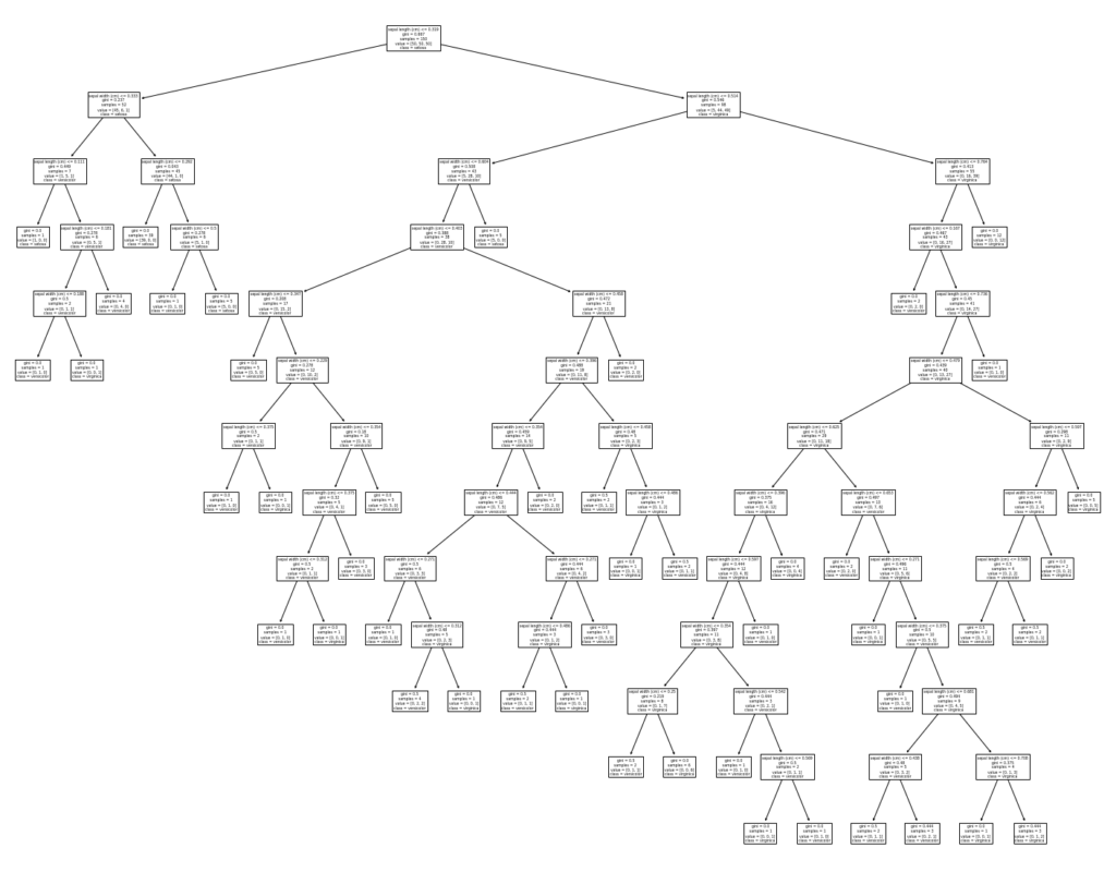
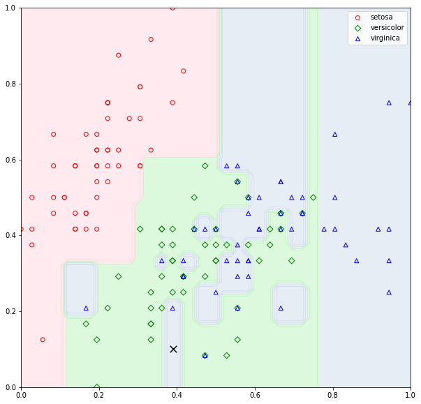
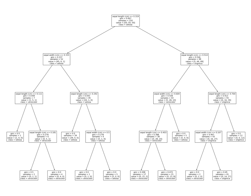
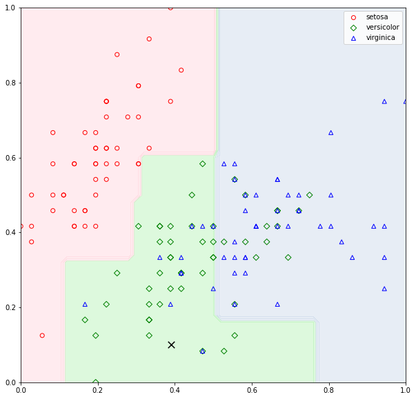
The algorithm builds a decision tree with zero error (misclassification) because it will keep on splitting until all the nodes are composed of one class (pure leaf nodes). This may cause overfitting (the model to overfit the data). Figure 3 illustrates a decision tree classifier fitted with the iris dataset. As can be seen in the figure, the decision surface shows a few blue regions with a single data point. These decision boundaries are induced due to the algorithm continues splitting until all leaf nodes are pure. Consider a test point indicated by the black cross in Figure 4. The test point will be classified as VIRGINICA although the test point falls in the region where the majority of the data points belong to VERSICOLOR. To prevent overfitting when building the tree, we can limit the number of splits in the tree structure which is known as pruning. In general, there are two approaches to tree pruning: pre-pruning and post-pruning.

Figure 4. A decision tree fitted with iris dataset and its decision boundaries.

Pre-pruning

In pre-pruning, we stop the tree-building process if the information gain of the split does not exceed a certain threshold. The threshold value is defined to justify the splitting of the node. In this way, the tree will not grow too large. We can also specify the maximum depth of the tree structure. The depth of the tree is defined by the maximum distance from the root node to a leaf node. Other common parameters that can be defined are the minimum number of instances required to split the node, the minimum number of instances to be a leaf and the maximum number of leaf nodes. Figure 5 shows a pruned decision tree by specifying the maximum depth to 4. The distance is counted by the number of paths from the root node to a leaf node. The decision boundaries of the tree are shown at the bottom of the figure. Although pre-pruning can prevent overfitting, fine-tuning the parameters is difficult and sometimes the obtained model is not optimal.

Figure 5. Pre-pruning the decision tree and its decision boundaries by limiting the number of splits.

Since the algorithm of building the tree is stopped before the misclassification rate is zero, some of the leaf nodes will not be pure. How do we assign which class to a leaf node? The leaf nodes are assigned to the class with the majority instances. For example, if leaf node $s$ composed of 5 instances belong to POSITIVE class and 2 instances belong to NEGATIVE class. Node $t$ will be assigned to POSITIVE class. The classification of a test point is given as follows:

$c = \arg \max_c p(y=c|t)$

where $p(y=c|\acute{x}, t)$ is predicted probability of class $c$ given the test point which is based on the proportion of instances belong to class $c$ in node $t$ . The probability of misclassification of leaf node $t$ is

$r(t) = 1 - \max_c p(y=c|t)$

Post-pruning

The post-pruning is to let the tree grow until the error rate is zero (full tree). Then, the size of the tree is reduced by removing the insignificant branches. This is known as cost-complexity pruning. In this method, we prune the tree by considering the error rate of the tree and the complexity of the tree. The tree complexity is defined as the number of leaf nodes. The higher the number of leaf nodes, the higher the complexity because the tree has more possibilities in partitioning the training set.

Specifically, the pruning method is governed by the cost-complexity measure. The function is to be minimized while pruning the tree. The function is given as follows:

$R_{\alpha}(T)=R(T) + \alpha \lvert \tilde{T} \rvert$

where $\lvert \tilde{T} \rvert$ is the tree complexity, $\alpha$ is the complexity parameter. $R(T)$ is the error rate of tree $T$ which is defined as follows:

$R(T)=r(t)p(t)$

where $r(t)$ is the probability of misclassification of leaf node $t$ . $p(t)=\frac{N(t)}{N}$ where $N(t)$ is number of instances in node $t$ and $N$ is the total number of instances.

$R(T)$ favors a larger tree because a large tree minimizes the error rate while $\lvert \tilde{T} \vert$ favors a smaller tree because a small tree minimizes the complexity of that tree.

The complexity parameter $\alpha$ governs the trade-off between the tree’s error rate and complexity. A large value of $\alpha$ results in a smaller tree while a small value of $\alpha$ results in a larger tree.

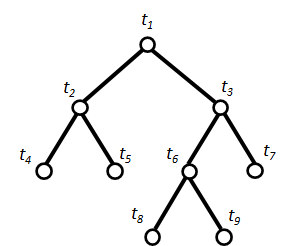
How do we determine which nodes are insignificant? Consider a tree structure in Figure 6. We look at any decision node and its two leaf nodes e.g. node $t_6$ and its two descendants, $t_8$ and $t_9$ . If the reduction in error when splitting $t_6$ is not significant, prune $t_8$ and $t_9$ and $t_6$ becomes the leaf node.

Figure 6. The error rate of the branch is less than its node.

Now, how do we evaluate the reduction in error? Based on the cost-complexity function, we can define the cost-complexity of a node, $t$ as follows:

$R_{\alpha}(t)=R(t) + \alpha$

For any node $t$ , in general, the error rate of its branch $T_t$ is less than or equals to its node.

$R(t) \geq R(T_t)$

where $R(T_t)=R(t_R)+R(t_L)$ . For example, consider node $t_6$ , the sum of error rate of $t_8$ and $t_9$ is less than or equals to the error of $t_6$ . Notice that the expression is parameterized by $\alpha$ . We know that when $\alpha$ is sufficiently small, $R(t) \geq R(T_t)$ is true. Therefore, if we choose a higher $\alpha$ , we will be able to know which decision node is the weakest link.

We can rewrite $R(t) \geq R(T_t)$ as follows:

$R(t) + \alpha \geq R(T) + \alpha \lvert \tilde{T} \vert$

Solving for $\alpha$ yields

$\alpha \leq \frac{R(T) - R(t)}{1-\lvert \tilde{T} \vert}$

The weakest link in a tree is

$\alpha(t) = \frac{R(T) - R(t)}{1-\lvert \tilde{T} \vert}$

where $R(T)$ is the error rate of tree $T$ , $R(t)$ is the error rate of node $t$ and $\lvert \tilde{T} \vert$ is the number of leaf nodes in $T$ .

Therefore, a decision node with the lowest $\alpha$ is the weakest link and its branch should be pruned. Then, the process is repeated on the pruned tree, until there is only the root node. By the end of this procedure, we have many subtrees. The optimal tree is selected among the subtrees using a validation set or cross-validation.

Numerical Example

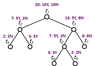
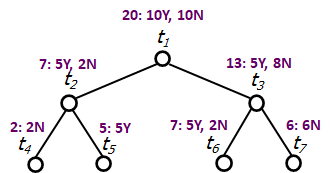
Consider a tree structure in Figure 7. The training set consists of 10 instances belonging to YES and 10 instances belonging to NO.

Figure 7. A decision tree fitted with 20 instances (10 YES and 10 NO).

Node $t_1$

$R(t_1)=\frac{10}{20} \cdot \frac{20}{20} = \frac{1}{2}$

$R(T_{t_1})=0$ (all leaf nodes are pure)

$\alpha(t_1) = \frac{\frac{1}{2} - 0}{5-1} = 0.125$

Node $t_2$

$R(t_2)=\frac{2}{7} \cdot \frac{7}{20} = \frac{1}{10}$

$R(T_{t_2})=0$ (all leaf nodes are pure)

$\alpha(t_2) = \frac{\frac{1}{10} - 0}{2-1} = 0.100$

Node $t_3$

$R(t_3)=\frac{5}{13} \cdot \frac{13}{20} = \frac{1}{4}$

$R(T_{t_3})=0$ (all leaf nodes are pure)

$\alpha(t_3) = \frac{\frac{1}{4} - 0}{3-1} = 0.125$

Node $t_6$

$R(t_6)=\frac{2}{7} \cdot \frac{7}{20} = \frac{1}{10}$

$R(T_{t_6})=0$ (all leaf nodes are pure)

$\alpha(t_6) = \frac{\frac{1}{10} - 0}{2-1} = 0.100$

Cost-complexity measure for each node.

$\alpha(t_1)=0.125$

$\alpha(t_2)=0.100$

$\alpha(t_3)=0.125$

$\alpha(t_6)=0.100$

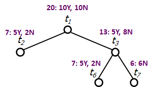
$\alpha(t_6)=0.100$ is minimum, hence we prune $t_8$ and $t_9$ ( $t_6$ has fewer instances than $t_2$ ). The subtree $T_1$ is given in Figure 8.

Figure 8. The pruned tree after first iteration.

Node $t_1$

$R(t_1)=\frac{10}{20} \cdot \frac{20}{20} = \frac{1}{2}$

$R(T_{t_1})=\frac{2}{20}$ (all leaf nodes are pure)

$\alpha(t_1) = \frac{\frac{1}{2} - \frac{2}{20}}{4-1} = 0.133$

Node $t_2$

$R(t_2)=\frac{2}{7} \cdot \frac{7}{20} = \frac{1}{10}$

$R(T_{t_2})=0$ (all leaf nodes are pure)

$\alpha(t_2) = \frac{\frac{1}{10} - 0}{2-1} = 0.100$

Node $t_3$

$R(t_3)=\frac{5}{13} \cdot \frac{13}{20} = \frac{1}{4}$

$R(T_{t_3})=\frac{2}{20}$ (all leaf nodes are pure)

$\alpha(t_3) = \frac{\frac{1}{4} - \frac{2}{20}}{2-1} = 0.150$

Cost-complexity measure for each node.

$\alpha(t_1)=0.125$

$\alpha(t_2)=0.100$

$\alpha(t_3)=0.125$

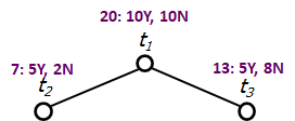
$\alpha(t_2)=0.100$ is minimum, hence we prune $t_4$ and $t_5$ . The subtree $T_2$ is given in Figure 9.

Figure 9. The pruned tree after second iteration.

Repeat the computation for each node.

Cost-complexity measure for each node.

$\alpha(t_1)=0.150$

$\alpha(t_3)=0.150$

$\alpha(t_3)=0.150$ is minimum, hence we prune $t_6$ and $t_7$ ( $t_3$ has fewer instances than $t_1$ ). The subtree $T_3$ is given in Figure 10.

Figure 10. The pruned tree after third iteration.

Repeat the computation for each node.

Cost-complexity measure for each node.

$\alpha(t_1)=0.150$

We prune $t_2$ and $t_3$ (there is only one node).

For each subtree, we evaluate their performance using a validation set or cross-validation. The optimal tree is the one with the highest accuracy or lowest error.

References

[1] L. Breiman, J. H. Friedman, R. A. Olshen, and C. J. Stone, Classification And Regression Trees. New York: Routledge, 2017. doi: 10.1201/9781315139470.