Hierarchical Agglomerative Clustering

Introduction

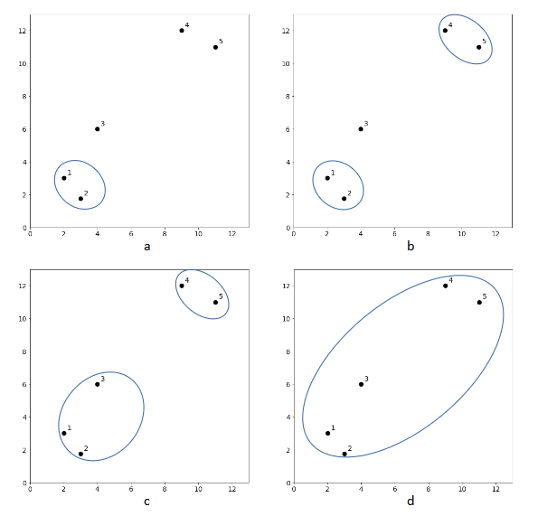
The clustering results of k-means algorithm depend on the value of k and the results may vary from one clustering to another. Unlike k-means, hierarchical agglomerative clustering is a clustering algorithm that does not require a pre-specified number of clusters. The algorithm begins with every data point representing a singleton cluster, in other words, there will be $N$ number of clusters. Then, the algorithm recursively merges a pair of clusters with the closest distance until all data points are merged into a single cluster. The iterative process is illustrated in Figure 1. There are five data points whereby each represents a singleton cluster. At each iteration, two closest clusters are merged into a single cluster, resulting in one less cluster. For example, in Figure 1a, cluster 1 and cluster 2 are merged since those two are the closest pair. This step produces one less cluster (cluster 1-2, cluster 3, cluster 4 and cluster 5). In the next iteration, cluster 4 and cluster 5 are the closest pair, hence the clusters are merged as shown in Figure 1b. This process is repeated until all clusters are merged.

Figure 1. Data points are iteratively merged based on the distance between the clusters.

Dendrogram

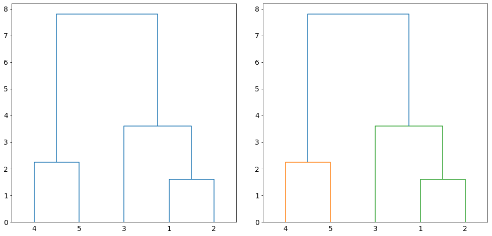
The iterative process produces a hierarchical representation in which the clusters at each level of the hierarchy are created. The hierarchical representation is called dendrogram. Figure 2 on the left shows the dendrogram of clustering the data points in Figure 1. A dendrogram is a tree-like structure representing the order of the cluster merging process. The leaf nodes (numbers at the bottom of the figure) are the initial clusters. The horizontal lines connecting the clusters indicate the merging of two pair of clusters. Furthermore, the lines shows the sequence at which the clusters are merged at every level (iteration) with the connected lines at the bottom indicate the first in sequence while the connected lines at the top is the last pair of clusters to be merged. The height of lines is proportional to the distance between the clusters. Clustering of a given size is induced if we cut the dendrogram at any given height. For example, if we cut at 5.0, two clusters will be induced as shown in Figure 2 on the right.

Linkage

The distances between the clusters in the above the example are computed using single linkage or also known as nearest neighbor linkage. Single linkage defines the distance between two clusters $G$ and $H$ as the minimum distance between two data points in $G$ and $H$ .

$d_{SL}(G,H)=\min_{x\in G, z\in H} d(x,z)$

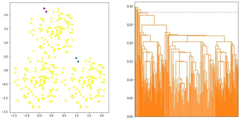
where $d(x,z)$ is the euclidean distance. Single linkage defines the distance by considering only a pair of closest data points from two clusters regardless of the similarity of the other data points of the clusters. This has the effect of “chaining” whereby the algorithm tends to merge two clusters if two data points from these clusters are close enough regardless of the other data points in the clusters. As a result, the clusters that will be formed are not compact or having high within-cluster variation as shown in Figure 3.

Figure 3. Dendrogram of single linkage agglomerative clustering.

Complete linkage is the opposite of single linkage whereby the distance between two clusters is determined by the maximum distance between two points in $G$ and $H$ .

$d_{CL}(G,H)=\max_{x\in G, z\in H} d(x,z)$

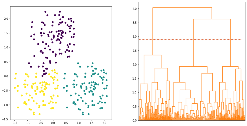
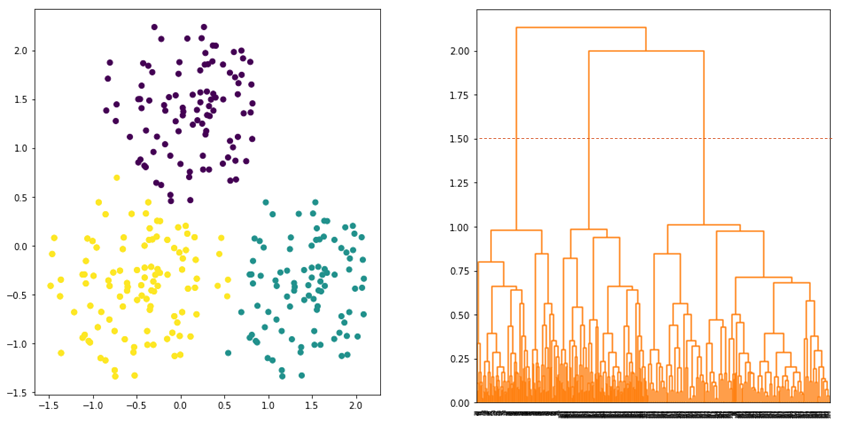
Since the linkage is defined by the maximum distance, two clusters are considered close (or merged) if the data points in the clusters are relatively similar. Thus, the algorithm tends to produce a more compact clusters. However, data points assigned to a cluster could be closer to data points of other clusters than they are to some data points of their own cluster. As shown in Figure 4, some data points that are assigned to PURPLE cluster are closer to YELLOW cluster.

Figure 4. Dendrogram of complete linkage agglomerative clustering.

Average linkage defines the distance between two clusters by calculting the average distance between all data points in the clusters. The linkage is defined as follows:

$d_{AL}(G,H)=\frac{1}{N_G \dot N_H} \sum_{x\in G, z\in H} d(x,z)$

where $N_G$ and $N_H$ are the number of data points in cluster $G$ and $H$ . Average linkage tries to strike a balance whereby all data points in the clusters contribute equally in determining the distance between the clusters. Hence, the clusters tend to be more compact and far apart as shown in Figure 5.

Figure 5. Dendrogram of average linkage agglomerative clustering.

Ward linkage is another linkage that produces a good clustering result. The linkage defines the distance between two clusters by considering the increase in variance when the clusters are merged. Ward linkage is defined as follows:

$\begin{aligned}d_{WL}(G,H) &=\sum_{x\in G \cup H} d(x,\mu_{G \cup H}) - \sum_{x \in G} d(x,\mu_G) - \sum_{x \in H} d(x,\mu_H) \\ &= \frac{N_G N_H}{N_G+N_H}d(\mu_G,\mu_H) \end{aligned}$

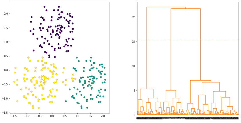
where $N_G$ and $N_H$ are the number of data points in cluster $G$ and $H$ . Instead of calculating the distance between the data points, ward linkage calculates the distance between the data points and the centroid of the clusters. Hence, the clusters are compact and far apart as shown in Figure 6.

Figure 6. Dendrogram of ward linkage agglomerative clustering.

Numerical Example

Consider the following set of data points.

$\mathbf{x}=\begin{bmatrix} 1.0&1.0 \\ 1.5&1.5 \\ 5.0&5.0 \\3.0&4.0 \\ 4.0&4.0 \\ 3.0&3.5 \end{bmatrix}$

Suppose we use complete linkage.

Calculate the distance between the data points. The distance matrix is given as follows:

	$x_1$	$x_2$	$x_3$	$x_4$	$x_5$	$x_6$
$x_1$	0.00	0.71	5.66	3.61	4.24	3.20
$x_2$	0.71	0.00	4.95	2.92	3.54	2.50
$x_3$	5.66	4.95	0.00	2.24	1.41	2.50
$x_4$	3.61	2.92	2.24	0.00	1.00	0.50
$x_5$	4.24	3.54	1.41	1.00	0.00	1.12
$x_6$	3.20	2.50	2.50	0.50	1.12	0.00

where the first row lists the distances between $x_1$ and other data points, second row lists the distances between $x_2$ and other data points, etc.

Merge two closest clusters. We merge $x_4$ and $x_6$ since their distance is minimum (closest). Then, complete linkage is used to determine the distance between $x_{4-6}$ and other data points. The distance matrix is given as follows:

	$x_1$	$x_2$	$x_3$	$x_{4-6}$	$x_5$
$x_1$	0.00	0.71	5.66	3.61	4.24
$x_2$	0.71	0.00	4.95	2.92	3.54
$x_3$	5.66	4.95	0.00	2.50	1.41
$x_{4-6}$	3.61	2.92	2.50	0.00	1.12
$x_5$	4.24	3.54	1.41	1.12	0.00

We repeat the process. Merge two closest clusters. We merge $x_1$ and $x_2$ since their distance is minimum (closest). Then, complete linkage is used to determine the distance between $x_{1-2}$ and other data points. The distance matrix is given as follows:

	$x_{1-2}$	$x_3$	$x_{4-6}$	$x_5$
$x_{1-2}$	0.00	5.66	3.61	4.24
$x_3$	5.66	0.00	2.50	1.41
$x_{4-6}$	3.61	2.50	0.00	1.12
$x_5$	4.24	1.41	1.12	0.00

We repeat the process. Merge two closest clusters. We merge $x_{4-6}$ and $x_5$ since their distance is minimum (closest). Then, complete linkage is used to determine the distance between $x_{4-5-6}$ and other data points. The distance matrix is given as follows:

	$x_{1-2}$	$x_3$	$x_{4-5-6}$
$x_{1-2}$	0.00	5.66	4.24
$x_3$	5.66	0.00	2.50
$x_{4-5-6}$	4.24	2.50	0.00

We repeat the process. Merge two closest clusters. We merge $x_{3}$ and $x_{4-5-6}$ since their distance is minimum (closest). Then, complete linkage is used to determine the distance between $x_{3-4-5-6}$ and $x_{1-2}$ . The distance matrix is given as follows:

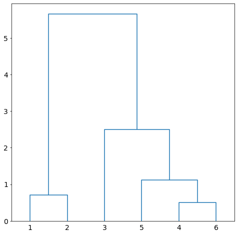
We repeat the process. Merge $x_{1-2}$ and $x_{3-4-5-6}$ since there are two clusters only. The dendrogram of the clustering is given in Figure 7.

Figure 7. The dendrogram of complete linkage agglomerative clustering.

Suppose we use average linkage.

Calculate the distance between the data points. The distance matrix is given as follows:

	$x_1$	$x_2$	$x_3$	$x_4$	$x_5$	$x_6$
$x_1$	0.00	0.71	5.66	3.61	4.24	3.20
$x_2$	0.71	0.00	4.95	2.92	3.54	2.50
$x_3$	5.66	4.95	0.00	2.24	1.41	2.50
$x_4$	3.61	2.92	2.24	0.00	1.00	0.50
$x_5$	4.24	3.54	1.41	1.00	0.00	1.12
$x_6$	3.20	2.50	2.50	0.50	1.12	0.00

	$x_1$	$x_2$	$x_3$	$x_{4-6}$	$x_5$
$x_1$	0.00	0.71	5.66	3.41	4.24
$x_2$	0.71	0.00	4.95	2.21	3.54
$x_3$	5.66	4.95	0.00	2.37	1.41
$x_{4-6}$	3.41	2.21	2.37	0.00	1.10
$x_5$	4.24	3.54	1.41	1.10	0.00

We repeat the same process until all clusters are merged into a single cluster.