Logistic Regression – Halim Noor

Introduction

Logistic regression is a parametric algorithm for solving classification problems whereby the label, $y\in{\{0,1\}}$ . Logistic regression and perceptron are similar whereby a hyperplane is defined to divide the feature space into regions labeled according to the classification. The hyperplane is defined by the inner product between parameters the and the input vectors (summation of the weighted inputs), $\mathbf{w}^T\mathbf{x}$ . Then, the resultant of the inner product is passed to a function that ensures the predicted value to be $0 \leq \hat{f}(\mathbf{x}) \leq 1$ via

$\hat{f}(\mathbf{x})=\text{sigm}(\mathbf{w}^T\mathbf{x})$

$\text{sigm}(z)$ refers to the sigmoid function, also known as logistic function which is defined as

$\text{sigm}(z)=\frac{1}{(1+e^{-z})}$

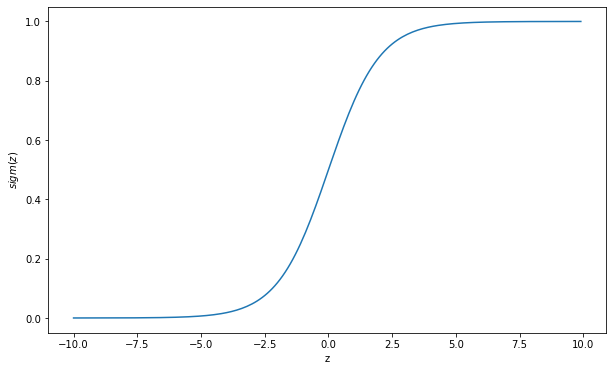
Figure 1 shows the graph of the sigmoid function. The sigmoid function has an S-shaped curve, which maps its input to a value within the range of 0 and 1. Thus, logistic regression has a probabilistic connotation. The curve has two horizontal asymptotes, one end is approaching 1 and the other end is approaching 0. Due to this property, the sigmoid function is differentiable at every point.

Figure 1. The sigmoid function is over -10 to +10.

As mentioned above, a logistic regression model outputs values within the range of 0 and 1. If we threshold the output at 0.5, a classification rule can be defined as follows:

$\hat{f}(\mathbf{x}) = \begin{cases} 1 & \text{sigm}(z) > 0.5 \\ 0 & \text{sigm}(z) \leq 0.5 \end{cases}$

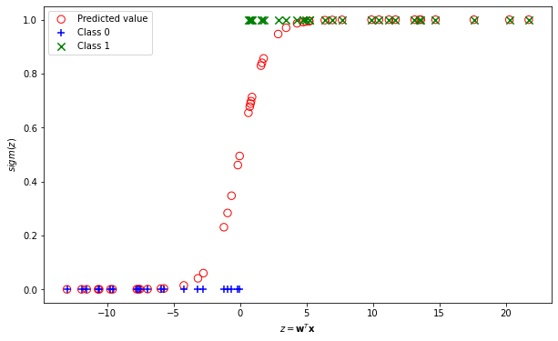
Figure 2 shows the output probabilities of 50 simulated inputs to the sigmoid function. The input values vary from -17 to +22 and their predicted values are indicated by the red circles. Using a threshold value of 0.5, the classification of the data is indicated by the green and blue markers. As can be seen in the figure, output probabilities above the threshold value are classified as 1. Otherwise, they are classified as 0.

Figure 2. The output probabilities of the sigmoid function and their classification using a threshold value of 0.5.

Numerical Example

Consider the logistic regression model $\hat{f}(\mathbf{x})=g(z)$ where $z=-4+x_1+x_2$ . Predict the labels of the following inputs.

$\mathbf{x}=\begin{bmatrix} 1&1\\1.5&1\\ 3&3\\3&4 \end{bmatrix}$

$z^1 = -4 + 1 + 1 = -2$ , $g(z^1) = \frac{1}{1+e^{2}} = 0.119$ , $\hat{y}^1 = 0$

$z^2 = -4 + 1.5 + 1 = -1.5$ , $g(z^2) = \frac{1}{1+e^{1.5}} = 0.182$ , $\hat{y}^2 = 0$

$z^3 = -4 + 3 + 3 = 2$ , $g(z^3) = \frac{1}{1+e^{-2}} = 0.881$ , $\hat{y}^3 =1$

$z^4 = -4 + 3.5 + 3 = 3$ , $g(z^4) = \frac{1}{1+e^{-3}} = 0.953$ , $\hat{y}^4 =1$

Multiclass Classification Setting

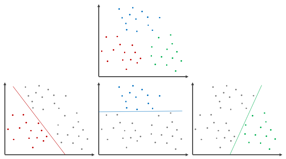
So far, we have seen logistic regression for binary classification. Real-world problems may involve more than two classes. For multiclass classification, we need to train multiple logistic regression models, one for each of the $C$ classes. For example, consider a classification problem as illustrated in Figure 3 (top). The data points belong to three classes, RED, BLUE and GREEN. We build three logistic regression models for each of the three classes. First, we treat RED instances as class 1, and all the other instances as class 0. Then, we build the logistic regression model to distinguish RED instances from the rest. Next, we treat BLUE instances as class 1 and all the other instances as class 0, and build the logistic regression model to distinguish BLUE instances from the rest. We perform the same method for GREEN instances. Eventually, we have three logistic regression models as shown in Figure 3 (bottom).

Given a test point, $\mathbf{\acute{x}}$ , all models perform the prediction on the test point and produce $C$ predicted values.

$\hat{f}_c(\mathbf{\acute{x}})=\mathbf{w}_c^T\mathbf{\acute{x}}$

Then, the predicted values are normalized using the softmax function. The softmax function turns the predicted values into probabilities. Each predicted value will be in the range of 0 and 1 and the sum of the values equal to 1.

$\hat{f}_c(\mathbf{\acute{x}})=\frac{e^{\hat{f}_c(\mathbf{\acute{x}})}} {\sum_{k=1}^C e^{\hat{f}_k(\mathbf{\acute{x}})} }$

The test point is assigned to the class with the largest probability.

Figure 3. Logistic regression in a multiclass classification setting.

Parameter Estimation

Now, how do we estimate the parameters of the logistic regression? We will discuss the estimation of the parameters for two-class logistic regression to simplify the explanation. The loss function of logistic regression is the negative log-likelihood or cross entropy as follows:

$J(\mathbf{w})=- \sum_{i=1}^N y^i \log{\hat{y}^i} + (1-y^i) \log{(1-\hat{y}^i)}$

where $\hat{y}^i = \hat{f}(\mathbf{x}^i) = \sigma (z^i)$ , $\sigma$ denotes the sigmoid function and $z^i=\mathbf{w}^T \mathbf{x}^i$

We take the derivative of the loss function with respect to the parameters and set to zero. Using chain rule, the derivate of the loss function is

$\frac{\partial J}{\partial w_j} = \sum_{i=1}^{N} \frac{\partial J}{\partial \hat{y}^i} \cdot \frac{\partial \hat{y}^i}{\partial z^i} \cdot \frac{\partial z^i}{\partial w_j}$

$\frac{\partial J}{\partial w_j} = \sum_{i=1}^{N} \frac{\hat{y}^i-y^i}{\hat{y}^i (1-\hat{y}^i)} \hat{y}^i(1-\hat{y}^i)x_j^i = \sum_{i=1}^{N} (\hat{y}^i-y^i) x_j^i$

$\sum_{i=1}^{N} (\hat{y}^i-y^i) x_j^i=0$

However, the maximum likelihood estimation of the parameters are not in closed form. Thus, the equation needs to be solved using optimization algorithm such as gradient descent, Newton’s method etc. Using gradient descent, the parameters are estimated as follows:

$\mathbf{w} := \mathbf{w} - \alpha \mathbf{g}$

where $\alpha$ is the learning rate and $\mathbf{g}=\frac{\partial J}{\partial \mathbf{w}}$ is the gradient or the derivative of the loss function with respect to the parameters.

Gradient Computation for Multinomial Logistic Regression

We show the gradient computation for multinomial logistic regression. The loss function is the negative log-likelihood.

$J(\mathbf{w}) = - \sum_{i=1}^{N} \sum_{k=1}^{C} (y_k^i \log{\hat{y}_k^i} )$

The probabilistic outputs are calculated using the softmax function. The probability of class $l$ is given as follows:

$\hat{y}_k = \frac{e^{z_k}} {\sum_{l=1}^C e^{z_l} }$

where $z_k = \mathbf{w}_k^T\mathbf{x}$ .

The gradient with respect to $w_{k,j}$ is

$\frac{\partial J}{\partial w_{k,j}} = \sum_{i=1}^{N} \frac{\partial J}{\partial \hat{y}_k^i} \cdot \frac{\partial \hat{y}_k^i}{\partial z_k^i} \cdot \frac{\partial z_k^i}{\partial w_{k,j}}$

The derivative of the loss function is

$\frac{\partial J}{\partial \hat{y}_k} = -\frac{y_k}{\hat{y}_k}$

The derivative of softmax $\frac{\partial \hat{y}_k}{\partial z_k}$ is given as follows. From quotient rule, we know that

$f'(x) = \frac{g'(x)h(x)-h'(x)g(x)}{h(x)^2}$

The computation of the derivative has two cases: $l=k$ and $l \neq k$ .

For $l=k$

$\begin{aligned} \frac{\partial \hat{y}_k}{\partial z_l} &= \frac{e^{z_k} \sum - e^{z_l} e^{z_k}}{\sum^2} \\ &= \frac{e^{z_k} \sum}{\sum^2} - \frac{e^{z_l} e^{z_k}}{\sum^2} \\ &= \hat{y}_k - \hat{y}_k^2 \\ &= \hat{y}_k(1-\hat{y}_k) \end{aligned}$

where $\sum = \sum_{l=1}^{C} e^{z_l}$

The derivative of the summation of the weighted inputs is

$\frac{\partial z_k}{\partial w_{k,j}} = x_{j}$

Therefore, the gradient is

$\begin{aligned} \frac{\partial J}{\partial w_{k,j}} &= -\frac{y_k}{\hat{y}_k} \cdot \hat{y}_k(1-\hat{y}_k) \cdot x_{j} \\ &= -y_k (1- \hat{y}_k)x_{j} \end{aligned}$

For $l \neq k$

$\begin{aligned} \frac{\partial \hat{y}_k}{\partial z_l} &= \frac{0 - e^{z_l} e^{z_k}}{\sum^2} \\ &= - \hat{y}_l \hat{y}_k \end{aligned}$

where $\sum = \sum_{l=1}^{C} e^{z_l}$

The derivative of the summation of the weighted inputs is

$\frac{\partial z_k}{\partial w_{k,j}} = x_{j}$

Therefore, the gradient is

$\begin{aligned} \frac{\partial J}{\partial w_{k,j}} &= -\frac{y_k}{\hat{y}_k} \cdot -\hat{y}_l \hat{y}_k \cdot x_{j} \\ &= y_k \hat{y}_l x_{j} \end{aligned}$

Then, we add both gradients as follows:

$\begin{aligned} \frac{\partial J}{\partial w_{k,j}} &= \sum_{l \neq k} y_k \hat{y}_l x_{j} + -y_k (1- \hat{y}_k)x_{j} \\ &= (\sum_{l \neq k} y_k \hat{y}_l - y_k (1- \hat{y}_k) )x_{j} \\ &= (\sum_{l \neq k} y_k \hat{y}_l + y_k \hat{y}_k -y_k) )x_{j} \end{aligned}$

The terms $\sum_{l \neq k} y_k \hat{y}_l + y_k \hat{y}_k$ can be combined to become $\sum_k y_k \hat{y}_k$ . Thus,

$\frac{\partial J}{\partial w_{k,j}} = (\sum_k y_k \hat{y}_k -y_k) x_{j}$

We know that $\sum_k y_k = 1$ . Therefore

$\frac{\partial J}{\partial w_{k,j}} = (\hat{y}_k -y_k) x_{j}$