Perceptron – Halim Noor

Introduction

Perceptron is a parametric algorithm for solving binary classification problems whereby the label, $y\in{\{-1,+1\}}$ [1]. The assumption of perception is that data points are linearly separable. Specifically, we can define a hyperplane that can divide the feature space into regions and each region is labeled according to the classification. Although the assumption sounds simplistic, if data points belonging to a particular class have similar characteristics and are clustered together, the hyperplane can be defined between the clusters of the two classes to classify the data points.

Essentially, given an input vector, $\mathbf{x}=(x_1, x_2, …,x_d)$ , the perceptron is a linear model that predicts the labels via

$\hat{f}(\mathbf{x})=\text{sign}(w_0 + \sum_{j=1}^{d} w_jx_j)$

where $w_0$ is the intercept also known as bias and $w_jx_j$ is the inner product between the model’s coefficient (or weight) vector and the input vector also known as linear combination of the inputs. We can introduce a constant input, $x_0$ whose value is always 1. Then, the expression can be simplified as follows:

$\hat{f}(x)=\text{sign}(\sum_{j=0}^{d} w_jx_j)=\mathbf{w}^T\mathbf{x}$

where $\mathbf{w}^T\mathbf{x}$ is the inner product in vector form.

$\text{sign}(z)$ is the sign function which returns $+1$ if $z$ is positive value and returns $-1$ if $z$ is negative value. Thus, given a test input, $\acute{x}$ , the classification of the input is given as follows:

$\hat{f}(\acute{x})=\begin{cases} +1 & \mathbf{w}^T\mathbf{x}>0 \\ -1 & \mathbf{w}^T\mathbf{x}<0 \end{cases}$

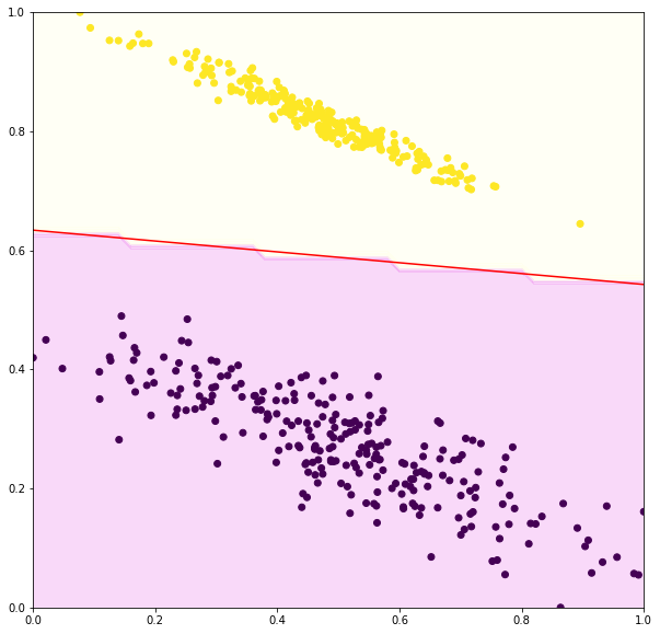
Consider a binary classification problem in Figure 1. The labels of the data points are YELLOW ( $+1$ ) and PURPLE ( $-1$ ). A perception model is fitted to those data points. The decision boundary is defined by $\mathbf{w}^T\mathbf{x}$ as indicated by the red line. The input space classified as $+1$ is denoted by the orange shaded region while the purple shaded region denotes the input space classified as $-1$ .

Figure 1. The decision boundary and regions of the perception are indicated by the red line and the shaded regions respectively.

Numerical Example

Consider the perception model $\hat{f}(\mathbf{x})=-4+x_1+x_2$ . Predict the labels of the following inputs.

$\mathbf{x}=\begin{bmatrix} 1&1\\1.5&1\\ 3&3\\3&4 \end{bmatrix}$

$\hat{f}(\mathbf{x}^1) = -4 + 1 + 1 = -2$ . $\hat{y}^1=-1$

$\hat{f}(\mathbf{x}^2) = -4 + 1.5 + 1 = -1.5$ . $\hat{y}^2=-1$

$\hat{f}(\mathbf{x}^3) = -4 + 3 + 3 = 2$ . $\hat{y}^3=+1$

$\hat{f}(\mathbf{x}^4) = -4 + 3.5 + 3 = 3$ . $\hat{y}^4=+1$

Algorithm

As shown above, the weights, $\mathbf{w}$ define the hyperplane that separates the data points. The algorithm to find the optimal weights is given as follows:

initialize weights, 
while :
  
  for each (,) in training set:
    
    if :

First, the weights are initialized randomly. The algorithm keeps training until all instances are correctly classified. Thus, if the data is not linearly separable, the training will loop forever. For each iteration, error, $e$ is initialized to zero, and the whole instances of the training set are classified and compared with their corresponding labels one by one. If the classification is incorrect, increment $e$ , and the weights are updated with values of element-wise multiplication $\odot$ between the instance and the label. Otherwise, the weights are not updated.

References

[1] F. Rosenblatt, “The Perceptron—a perceiving and recognizing automaton,” Cornell Aeronautical Laboratory, 1957.