Boosting – Halim Noor

Introduction

Boosting is an ensemble learning algorithm that combines many weak base models to produce a strong model. A weak model is a model that performs slightly better than random guessing. Thus, a weak model has an error rate that is slightly below 50%. The model could be any machine learning model such as a decision tree with a single split which is also known as decision stump. Unlike bagging models which consist of independent base models, boosting method sequentially builds the base models in which the models are trained based on the predictions of the previous models. We describe boosting in general first. The following sections present two popular boosting algorithms, adaptive boosting and gradient boosting.

Generally, a boosting model takes the form

$\hat{f}(\mathbf{x})=\sum_{m=1}^{M} \alpha_m b(\mathbf{x};\gamma_m)$

where $\alpha_m$ is the weight of base model $m$ . The ensemble model is built in an iterative manner whereby at iteration $m$ , we add base model $\alpha_m b(\mathbf{x};\gamma_m)$ to the ensemble model. The final prediction is obtained by evaluating all the base models and taking the weighted sum.

The training is an iterative process whereby base models are added sequentially to the ensemble boosting model. At each iteration $m$ , the base model and its corresponding optimal weight are solved and added to the ensemble, and this process is repeated for $M$ base models.

$\hat{f}_m(\mathbf{x}) = \hat{f}_{m-1}(\mathbf{x}) + \alpha_m b(\mathbf{x};\gamma_m)$

Typically, the optimal base model of each iteration is trained by minimizing a loss function.

$\min_{\alpha_m, \gamma_m} \sum_{i=1}^{N} L(y^i, \alpha_m b(\mathbf{x};\gamma_m))$

where $L$ is the loss function such as the squared loss and negative log-likelihood.

Adaptive Boosting

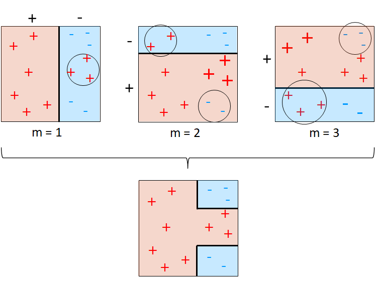
Adaptive boosting, or simply AdaBoost [1] sequentially trains the base models on weighted training instances in which the weights are also sequentially modified to indicate the importance of the instances in the training process. Initially, the instances have equal weights. In the following iteration, the weights of the instances are individually updated based on the predictions of the base model. Those instances that were incorrectly predicted have their weights increased, while the instances that were correctly predicted have their weights decreased. Thus, the weights of the instances that are difficult to predict correctly will be ever-increased as iterations proceed, forcing the subsequent base models to focus on those instances.

Figure 3 illustrates shows the training process of AdaBoost using a simple training set. As shown in the figure, the number of iterations is 3, hence the training process builds three base models. Initially, equal weight is assigned to each instance and the base model is trained in the usual manner. Then, the weights of the instances are adjusted so that the misclassified instances are given more importance in the next iteration. In iteration $m=1$ , the three misclassified positive instances as indicated by the circle have their weights increased. This is shown by the size of those instances in iteration $m=2$ . The same procedure is followed for iteration $m=3$ .

Figure 3. A series of base models are trained on weighted instances that are individually updated for every iteration.

We describe the formulation of AdaBoost for binary classification. Although AdaBoost was initially introduced for binary classification, it has been extended to multi-class classification and regression. In AdaBoost, the optimal weak model is solved using the exponential loss which is defined as follows.

$L(\hat{f}) = e^{-y \hat{f}(\mathbf{x})}$

Consider a dataset ${(\mathbf{x}^1,y^1),(\mathbf{x}^2,y^2),...,(\mathbf{x}^N,y^N)}$ where each target $y^i \in {-1,+1}$ . At iteration $m$ , we solve for the optimal weak model $b(\mathbf{x})$ and the corresponding weight $\alpha_m$ which to be added to the ensemble model using the exponential loss.

$\begin{aligned} \alpha_m, b_m &= \arg \min_{\alpha,b} \sum_{i=1}^{N} e^{-y^i (\hat{f}_{m-1}(\mathbf{x}^i) + \alpha b(\mathbf{x}^i))} \\ &=\arg \min_{\alpha,b} \sum_{i=1}^{N} e^{-y^i \hat{f}_{m-1}(\mathbf{x}^i)} e^{-\alpha y^i b(\mathbf{x}^i) } \end{aligned}$

Let $w_m^i=e^{-y^i \hat{f}_{m-1}(\mathbf{x}^i)}$ . Note that the term does not depend on $\alpha$ and $b$ , but depends on the ensemble model $\hat{f}_{m-1}$ . Thus, we can assume $w_m^i$ as the weight of instance $i$ at iteration $m$ .

$\alpha_m, b_m = \arg \min_{\alpha,b} \sum_{i=1}^{N} w_m^i e^{-\alpha y^i b(\mathbf{x}^i) }$

The expression can be written based on two cases: misclassification ( $y \neq b(\mathbf{x})$ ) and correct classification ( $y = b(\mathbf{x})$ ).

$\alpha_m, b_m = \arg \min_{\alpha,b} \sum_{i \vert y = b(\mathbf{x}) } w_m^i e^{-\alpha } + \sum_{i \vert y \neq b(\mathbf{x})} w_m^i e^{\alpha }$

We can write $\sum_{i \vert y = b(\mathbf{x}) } w_m^i e^{-\alpha } = \sum_{i=1}^{N} w_m^i e^{-\alpha } - \sum_{i \vert y \neq b(\mathbf{x}) } w_m^i e^{-\alpha }$ . Therefore, the above expression can be written as follows.

$\begin{aligned} \alpha_m, b_m &= \arg \min_{\alpha,b} \sum_{i=1}^{N} w_m^i e^{-\alpha} - \sum_{i \vert y \neq b(\mathbf{x}) } w_m^i e^{-\alpha } + \sum_{i \vert y \neq b(\mathbf{x})} w_m^i e^{\alpha } \\ &= \arg \min_{\alpha,b} e^{-\alpha } \sum_{i=1}^{N} w_m^i + \sum_{i \vert y \neq b(\mathbf{x})} w_m^i (e^{\alpha} - e^{- \alpha}) \\ &= \arg \min_{\alpha,b} (e^{\alpha} - e^{- \alpha}) \sum_{i=1}^{N} w_m^i I(y \neq b(\mathbf{x}^i)) + e^{-\alpha} \sum_{i=1}^{N} w_m^i \end{aligned}$

Assuming the instance weights have been normalized such that $\sum_{i=1}^{N} w_m^i = 1$ . The normalization factor is a constant factor, hence it will not affect the minimization operation.

$\alpha_m, b_m = \arg \min_{\alpha,b} (e^{\alpha} - e^{- \alpha}) \sum_{i=1}^{N} w_m^i I(y \neq b(\mathbf{x}^i)) + e^{-\alpha}$

From the above, since $e^{\alpha} - e^{- \alpha}$ is a positive value, we see that the weak base model $b_m$ to be added is

$b_m= \arg \min \sum_{i=1}^{N} w_m^i I(y \neq b(\mathbf{x}^i))$

We can see that this is actually the weighted error of the base model. Note that the base model doesn’t have to be strong. It is sufficient that the weighted error is less than 0.5.

Now, we need to solve for $\alpha_m$ . Let’s us denote the weighted error as $\epsilon_m = \sum_{i=1}^{N} w_m^i I(y \neq b(\mathbf{x}^i))$ . We substitute $\epsilon_m$ into the expression.

$\begin{aligned} \alpha_m &= \arg \min_{\alpha,b} (e^{\alpha} - e^{- \alpha}) \epsilon_m + e^{-\alpha} \\ &= \arg \min_{\alpha,b} e^{\alpha} \epsilon_m - e^{-\alpha} \epsilon + e^{-\alpha} \end{aligned}$

We take the derivative with respect to $\alpha$ , and then divide it by $e^{-\alpha}$ .

$\begin{aligned} \frac{\partial (e^{\alpha} \epsilon_m - e^{-\alpha} \epsilon + e^{-\alpha})}{\partial \alpha} &= e^{\alpha} \epsilon_m + e^{-\alpha} \epsilon_m - e^{-\alpha} \\ &= e^{2\alpha} \epsilon_m + \epsilon_m + 1 \end{aligned}$

Setting it to zero to solve for the minimum.

$\begin{aligned} e^{2\alpha} \epsilon_m + \epsilon_m + 1 &= 0 \\ e^{2\alpha} &= \frac{1-\epsilon_m}{\epsilon_m} \\ 2\alpha &= \ln \frac{1-\epsilon_m}{\epsilon_m} \\ \alpha_m &= \frac{1}{2} \ln \frac{1-\epsilon_m}{\epsilon_m} \end{aligned}$

Therefore, the ensemble model is then updated

$\hat{f}_{m+1}(\mathbf{x}) = \hat{f}_{m}(\mathbf{x}) + \alpha_m b_m(\mathbf{x})$

Recall that $w_m^i=e^{-y^i \hat{f}_{m-1}(\mathbf{x}^i)}$ . The weights of the next iteration is

$\begin{aligned} w_{m+1}^i &= e^{-y^i \hat{f}_m(\mathbf{x}^i)} \\ &= e^{-y^i (\hat{f}_{m-1}(\mathbf{x}^i) + \alpha_m b_m(\mathbf{x}^i)) } \\ &= e^{-y^i \hat{f}_{m-1}(\mathbf{x}^i)} \cdot e^{-y^i b_m(\mathbf{x}^i) \alpha_m} \\ &= w_m^i \cdot e^{-y^i b_m(\mathbf{x}^i) \alpha_m} \end{aligned}$

We can rewrite $-y^i b_m(\mathbf{x}^i) = 2 \cdot I(y^i \neq b_m(\mathbf{x}^i)) - 1$ . Thus, the weight update becomes

$\begin{aligned} w_{m+1}^i &= w_m^i \cdot e^{(2 \cdot I(y^i \neq b_m(\mathbf{x}^i)) - 1) \alpha_m} \\ &= w_m^i \cdot e^{\alpha_m 2 \cdot I(y^i \neq b_m(\mathbf{x}^i)) - \alpha_m} \\ &= w_m^i \cdot e^{\alpha_m 2 \cdot I(y^i \neq b_m(\mathbf{x}^i))} \cdot e^{-\alpha_m} \end{aligned}$

Notice that the term $e^{-\alpha_m}$ multiplies all the weights by the same value and it will be canceled out in the normalization step. Thus, it has no effect on the weight update and can be dropped.

Putting everything together, the algorithm of AdaBoost is given below.

Initialize the instance weights  where 
for  to M
   Train a base model  using the weighted training set.
   Compute 
   if 
      Compute 
      
      Set 
   else
      return 
Return

Gradient Boosting

Gradient boosting is a generalized boosting algorithm that is based on gradient descent. Recall that gradient descent is used to approximate the function (predictive model) by minimizing the loss function. This is done by computing the gradients of the loss function with respect to the weights which are then used to update the weights. Using the same approach, we can search the same way over functions instead of the weights [2-3].

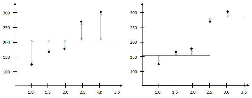
Consider a gradient boosting algorithm with $M$ steps. The algorithm begins with a random guessed function as the initial weak base model, which could be the average function as indicated by the black line in Figure 4. For each subsequent $m$ steps, we add a base model that will correct the error of its predecessor’s predictions. This is done by calculating the difference between the predictions and the true values as indicated by the blue line. The prediction error which is also known as residual, is then used as the target to train the base model and add it to the ensemble model. The reasoning behind this is that if we can approximate the residuals, we can use it to correct wherever errors it had made. This is shown in the figure on the right, the residuals have been reduced when the average function is added with the newly built base model.

Figure 4. The base model is trained on the residuals to improve the prediction.

We describe the formulation of gradient boosting for regression. Given a loss function

$L(\hat{f})=\sum_{i=1}^{N}L(y^i,\hat{f}(\mathbf{x}^i))$

where $L(y^i,\hat{f}(\mathbf{x}^i))$ is the regression loss such as squared loss function and $\hat{f}$ is the approximated function or the trained model. The aim is to minimize $L(\hat{f})$ with respect to $\hat{f}$ . Recall that in boosting, weak base models are sequentially added to produce an ensemble model. Thus, minimizing the loss function can be viewed as

$\mathrm{\hat{f}} = \arg \min L(\hat{f})$

where $\mathrm{\hat{f}} = (\hat{f}(\mathbf{x}^1),\hat{f}(\mathbf{x}^2),...,\hat{f}(\mathbf{x}^N) )$ . The optimization problem is solved using gradient descent. At step $m$ , the gradient of $L(\mathrm{\hat{f}})$ is

$g_m^i=[\frac{\partial L(y^i,\hat{f}(\mathbf{x}^i))}{\partial \hat{f}(\mathbf{x}^i)}]_{\hat{f}=\hat{f}_{m-1}}=-(y^i - \hat{f}(\mathbf{x}^i))$

We would like to reduce the residuals of the previous step. Thus the negative gradient is taken

$r_m^i= -g_m^i = (y^i-\hat{f}(\mathbf{x}^i))$

Train $b_m(\mathbf{x},\gamma_m)$ using the ${(\mathbf{x}^1,r^1),(\mathbf{x}^2,r^2),...,(\mathbf{x}^N,r^N)}$ .

$\gamma_m = \arg \min \sum_{i=1}^N (r_m^i - b(\mathbf{x}^i, \gamma))^2$

Finally, add $b_m$ to the ensemble model.

$\hat{f}_m = \hat{f}_{m-1} + \alpha b_m$

where $\alpha$ is a constant value typically in the range of 0 and 1.

In practice, the base model is implemented a decision tree with a limited depth e.g. maximum depth of 3. Gradient boosting can be used for both regression and classification. For classification, the log loss (binary cross entropy) is used as the loss function. Putting everything together, the algorithm of gradient boosting is given below.

for  to 
   Compute the gradient residual 
   Train a base model which minimize 
   Update 
Return

References

[1] Y. Freund and R. E. Schapire, “A Decision-Theoretic Generalization of On-Line Learning and an Application to Boosting,” Journal of Computer and System Sciences, vol. 55, no. 1, pp. 119–139, Aug. 1997, doi: 10.1006/jcss.1997.1504.

[2] J. H. Friedman, “Greedy Function Approximation: A Gradient Boosting Machine,” The Annals of Statistics, vol. 29, no. 5, pp. 1189–1232, 2001.

[3] J. H. Friedman, “Stochastic gradient boosting,” Computational Statistics & Data Analysis, vol. 38, no. 4, pp. 367–378, Feb. 2002, doi: 10.1016/S0167-9473(01)00065-2.