Attention

Encoder-Decoder

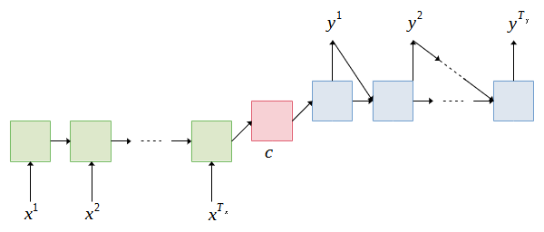
The most common network architecture for many-to-many sequence learning is called encoder-decoder [1-2]. The architecture is the basis of state-of-the-art machine translation models. In general, the encoder accepts the input sequence and encodes it into a feature representation of the input sequence which is known as a context vector. Then, the decoder takes the context vector and decodes it to produce the output sequence word by word. Figure 1 illustrates the block diagram of the encoder-decoder model.

Both encoder and decoder use recurrent neural network (RNN) to model the sequence of the data. The RNN may refer to the recurrent neural network or a variant of RNN such as LSTM and GRU. Let $\mathbf{x}$ of length $T_x$ denotes the source sequence and $\mathbf{y}$ of length $T_y$ denotes the target sequence. Note that the source and target variables are in bold to indicate they are vectors.

$\mathbf{x}=\{\mathbf{x}^1, \mathbf{x}^2,...,\mathbf{x}^{T_x}\}$

$\mathbf{y}=\{\mathbf{y}^1, \mathbf{y}^2,...,\mathbf{y}^{T_y}\}$

In the context of machine translation, the source is the set of sentences of to be translated and the target is the set of sentences of the language that we want to translate to. The RNN of the encoder reads the input sequence whereby at each time step, the inputs are the current word $\mathbf{x}^{t}$ and the hidden state from the previous time step $\mathbf{h}^{t-1}$ , and the output of the RNN is the new hidden state $\mathbf{h}^{t}$ . The initial hidden state of the decoder $\mathbf{h}^0$ is typically zeros. The encoder $f_{\texttt{enc}}$ can be represented as a function of $\mathbf{x}^{t}$ and $\mathbf{h}^{t-1}$ .

$\mathbf{h}^t = f_{\texttt{enc}}(\mathbf{x}^{t}, \mathbf{h}^{t-1})$

Once the final word of the input sequence is passed to the RNN, the final hidden state is used as the context vector $\mathbf{c}=\mathbf{h}^{T_x}$ . The context vector is passed to the decoder for decoding and generating the translation. The decoder is trained to generate the output or the target words $\mathbf{y}^t$ given hidden state $\mathbf{s}^t$ at each time step. Typically, fully connected layer(s) is used to predict the target words. The hidden state $\mathbf{s}^t$ is conditioned on the previous target word $\mathbf{y}^{t-1}$ and the previous hidden state $\mathbf{s}^{t-1}$ . The decoder $f_{\texttt{dec}}$ can be represented as follows.

$\mathbf{y}^t = f_{\texttt{dec}}(\mathbf{s}^t)$

where hidden state $\mathbf{s}^t$ is

$\mathbf{s}^t = g(\mathbf{y}^{t-1}, \mathbf{s}^{t-1})$ and $\mathbf{s}^0=\mathbf{c}$ .

We use two tokens to indicate the start and end of the source and target sentences: <start> and <end>. The tokens are appended to the start and end of the sequence $\mathbf{x}=\{\mathbf{x}^1,\mathbf{x}^2...,\mathbf{x}^{T_x}\}$ where $\mathbf{x}^1=<\texttt{start}>$ and $\mathbf{x}^{T_x}=<\texttt{end}>$ . Thus, the first input to the encoder and decoder is <start>. The subsequent inputs are the source and target words, and the last input <end>. When training the encoder-decoder model, we always know the number of words in the sequences. During inference, the model will keep generating the words until <end> token is generated.

In the previous section, we discussed encoder-decoder for sequence learning such as machine translation. In encoder-decoder model, the final hidden state of the encoder, also known as context vector is passed to the decoder for generating the target words. The context vector represents the compressed version of the input sequence. However, due to the fixed length of the context vector, the information needs to be compressed which may lead to information loss especially those early in the sequence. Bi-directional RNN may resolve the problem by processing the sequence in reverse order. However, the problem still persists when processing long input sequences. In [3], attention mechanism was introduced to solve the problem of learning long input sequences. Attention allows the model to attend on different “parts” of input sequences when generating the outputs at each time step. Unlike the standard encoder-decoder model, attention derives the context vector from the hidden states of both the encoder and decoder, and the alignment between the source and target.

The encoder is a bi-directional RNN that reads the sequence of inputs $\mathbf{x}=\{\mathbf{x}^1,\mathbf{x}^2,...,\mathbf{x}^{T_x}\}$ and generates forward hidden states $\overrightarrow{\mathbf{h}}$ and backward hidden states $\overleftarrow{\mathbf{h}}$ at each time step. The concatenation of the hidden states represents the encoder state.

$\mathbf{h} = [\overrightarrow{\mathbf{h}};\overleftarrow{\mathbf{h}}]$

where $\overrightarrow{\mathbf{h}}=\{ \mathbf{h}^1, \mathbf{h}^2,...,\mathbf{h}^{T_x} \}$ and $\overleftarrow{\mathbf{h}}=\{ \mathbf{h}^{T_x}, \mathbf{h}^{T_x-1},...,\mathbf{h}^1 \}$

At each time step, the decoder generates a hidden state as follows.

$\mathbf{s}^t = f(\mathbf{y}^t-1, \mathbf{s}^{t-1}, \mathbf{c}^t)$

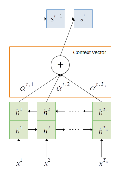
where the initial hidden state $\mathbf{s}^0=\overleftarrow{\mathbf{h}}$ , $\mathbf{c}^t$ is the context vector at time $t$ . The context vector is the summation of the hidden states of the encoder, weighted by alignment scores $\alpha^{t,j}$ as shown in Figure 2.

Figure 2. The context vector is derived by summing all the weighted hidden states of the encoder. Image is reproduced from [3].

$\mathbf{c}^t = \sum_j^{T_x} \alpha^{t,j} \mathbf{h}^j$

The alignment scores $\alpha^{t,j}$ are computed by

$\alpha^{t,j} = \frac{\texttt{exp}(\texttt{score}^{t,j} )}{ \sum_k^{T_x} \texttt{exp}(\texttt{score}^{t,k} ) }$

where $\texttt{score}^{t,j} = a(\mathbf{s}^{t-1},\mathbf{h}^j)$ .

The alignment scores are the measures of how well the input at position $j$ match the output at position $t$ . The scores are calculated based on the decoder hidden state $\mathbf{s}^t-1$ which is right before the output is generated and the encoder hidden state $\mathbf{h}^j$ .

Bahdanau et al. parameterize the alignment score function $a(\mathbf{s}^{t-1},\mathbf{h}^j)$ with fully connected layers that are jointly trained with the encoder and decoder. Specifically, the score function is defined as

$a(\mathbf{s}^{t-1},\mathbf{h}^j) = \mathbf{v}^\intercal \texttt{tanh}(\mathbf{w} \cdot \mathbf{s}^{t-1} + \mathbf{u} \cdot \mathbf{h}^j)$

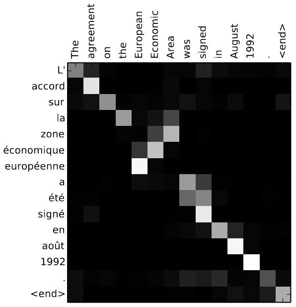
where $\mathbf{v}$ , $\mathbf{w}$ and $\mathbf{u}$ are weight matrices to be learned by the model. Figure 3 shows a sample of alignment scores calculated by the encoder-decoder model with attention for translating English words to French words.

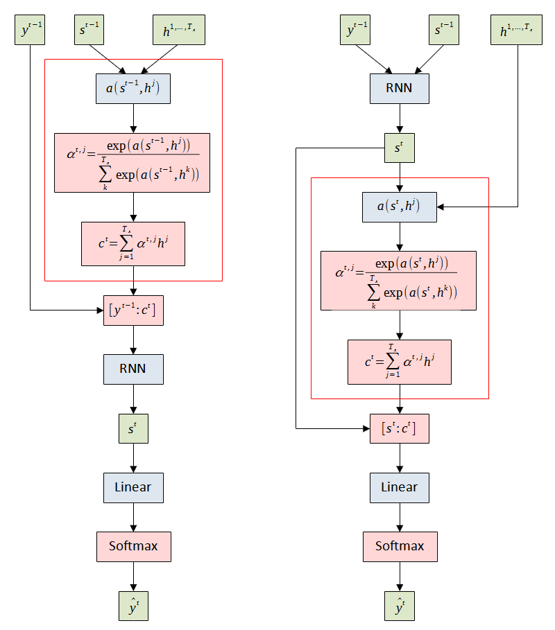
Figure 3. The alignment scores between the source words (English) and the generated translation (French). Image source from [3].

Given the significant improvement by integrating the attention mechanism, various forms of attention and alignment score functions have been introduced [4-5]. In [4], Luong et al. introduced several changes to generalize the attention mechanism which allows the alignment score function to be switched to different score functions. The key difference is the method of computing the context vector. Figure 4 illustrates the differences in the attention mechanisms. Bahdanau attention first derives the context vector. Then, the decoder feeds the concatenation of the context vector with the previous target word $\mathbf{y}^{t-1}$ to the decoder’s RNN to generate the current hidden state $\mathbf{s}^t$ . Luong attention first generates $\mathbf{s}^t$ using the decoder’s RNN and then uses it to derive the context vector. The decoder concatenates the context vector with $\mathbf{s}^t$ and feeds it to the fully-connected layer to generate the target word.

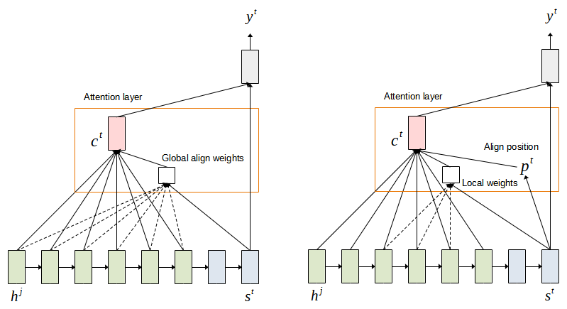
Figure 4. Bahdanau (left) and Luong (right) attention mechanisms. The red bounded box indicates the calculation of the context vector.

The attention that we discussed above attends to the entire hidden states of the encoder. This attention is called global attention model. This model has the drawback that it is computationally expensive for long sequences. Luong attention proposed the local attention model whereby the context vector is derived as a weighted average over a set of encoder hidden states $[p^t - D, p^t + D]$ where $D$ is empirically selected. The context vector is therefore calculated as follows. Figure 5 illustrates the computation of global and local attention.

$\mathbf{c}^t = \sum_{j=p^t-D}^{p^t+D} \alpha^{t,j} h^j$

Figure 5. Global and local attention. Encoder in green and decoder in blue. Images are reproduced from [4].

Another difference is that the encoder does not use a bi-directional recurrent neural network to simplify the computation. Thus, only forward hidden states are used when deriving the context vector. Finally, three alignment score functions are introduced: general, dot-product and location-based, as an alternative to the additive score function. Table 1 lists the popular attention mechanism and their alignment score functions.

\texttt{score}^{t,j} = \mathbf{v}^\intercal \texttt{tanh}(\mathbf{w} \cdot \mathbf{s}^{t-1} + \mathbf{u} \cdot \mathbf{h}^j) — Table 1. Popular alignment score functions.

\texttt{score}^{t,j} = \mathbf{h}^{j\intercal} \mathbf{w} \mathbf{s}^t — Table 1. Popular alignment score functions.

Self-Attention

Recurrent neural network is an essential component in attention model for learning sequential data. However, due to the sequential nature of recurrent neural network, it precludes parellization within the training data. For a sequence with $L$ lengths, the model needs to perform $O(n)$ sequential operations to generate the output sequence. The problem is becoming more pronounced when processing long input sequences.

The motivation of the development of self-attention is to reduce the computational complexity of the attention model. Like attention which allows the model to focus attention on specific parts of the input sequence, self-attention enables interaction between words in the sequence to compute the context vector, resulting in better capturing of the syntactic and semantic structure of the sentences.

The Transformer

The Transformer architecture proposed in [6] is the first model that relied entirely on self-attention for the alignment between input and output sequence without the recurrent architecture. Although the model does not use recurrent and convolutional layers, it retains the popular encoder-decoder architecture as shown in Figure 6. The encoder (on the left side of the figure), consists of six (6) identical layers whereby each has two sub-layers. The first sub-layer is multi-head attention which we will be explained later. The second sub-layer is position-wise feed forward network. The position-wise feed forward network is implemented using two fully-connected layers with ReLU activation function in between.

$\texttt{FFN}(\mathbf{x}) = \texttt{max}(0,\mathbf{x} \cdot \mathbf{W}_1 + b_1)\mathbf{W}_2 + b_2$

The sub-layers have a residual connection followed by layer normalization, that is the output of each sub-layer is

$y = \texttt{LayerNorm(x + \texttt{Sublayer(x)})}$

where $\texttt{Sublayer(x)}$ is the output of the sub-layer itself. All sub-layers and the embedding layer produce outputs of dimension $d_m=512$ .

Figure 6. The Transformer architecture consists of encoder (left) and decoder (right). Image source from [6].

The decoder as shown on the right side of the figure is also consists of six (6) identical layers. Each layer has two sub-layers as in the encoder and a third sub-layer, which also performs multi-head attention. This sub-layer receives one input from the first multi-head attention and two inputs from the encoder stack. Similar to the sub-layers of the encoder, a residual connection followed by layer normalization. The output of the decoder is passed to a fully-connected layer with softmax function for prediction.

Since the Transformer does not use any recurrent layer, it needs method to “know” the order of the words in the sequence. This is achieved by adding the positional encoding to create positional vectors which to be added to the input vectors. The positional encoding uses the sine and cosine functions of different frequencies to create the positional vectors.

$\texttt{PE}(p,2i) = \texttt{sin}(\frac{p}{1000^{\frac{2i}{d_m}}})$

$\texttt{PE}(p,2i+1) = \texttt{cos}(\frac{p}{1000^{\frac{2i}{d_m}}})$

where $p$ is the position and $i$ is the dimension.

Multi-head Attention

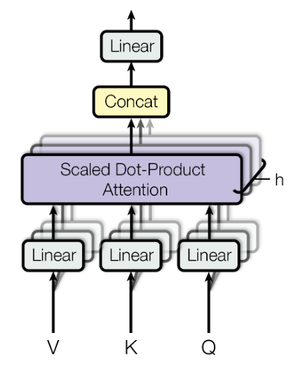
The multi-head attention consists of several components, of which the main component is the scaled dot-product attention as shown in Figure 7. The multi-head attention accepts three inputs denoted by $\mathbf{Q}$ , $\mathbf{K}$ and $\mathbf{V}$ , representing query, key and value vectors. The query and key have the same dimension $d_k$ and value has $d_v$ dimension. Note that the vectors may have the same dimension $d_k = d_v$ . Each vector is passed to a fully-connected layer, for linear projection.

$\mathbf{Q} = \mathbf{w}_q^{\intercal} \mathbf{x}$

$\mathbf{K} = \mathbf{w}_k^{\intercal} \mathbf{x}$

$\mathbf{V} = \mathbf{w}_v^{\intercal} \mathbf{x}$

where $\mathbf{w}_q$ , $\mathbf{w}_k$ and $\mathbf{w}_v$ are weight matrices to be learned. $\mathbf{Q}=\mathbb{R}^{m \times d_k}$ , $\mathbf{K}=\mathbb{R}^{m \times d_k}$ and $\mathbf{V}=\mathbb{R}^{m \times d_v}$ where $m$ is the length of sequence.

Figure 7. Multi-head attention, image source from [6].

The scaled dot-product attention computes the attention scores of the words. The sequence alignment is treated as a mapping between a query and a set of key-value pairs, and an output. The concept of query, key and value in self-attention is similar to the regular python dictionary. The following is a python dictionary with three keys and three values. A single query is passed to the dictionary to fetch some information. The query is a request for information, key is what kind of information the dictionary has and value is the information the dictionary has. When the query is passed to the dictionary, the search engine will map the query against a set of keys and return the information that the matching key is associated with. In the context of machine translation, the query is the target sequence, value is the source sequence and key is some information associated with the source sequence.

Courses = {'CPT111': 'Programming 1' , 'CPT112': 'Mathematic', 'CPT113': 'Programming 2'}
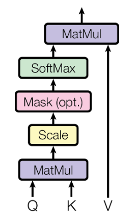
result = Courses['CPT112']

The query, key and value vectors are derived from the same item in the input sequence. Using these vectors, the output is calculated by adding the weighted values, where the weights are determined by how well the query matches the associated keys. The attention weights (or scores) are calculated as follows. We compute the dot products between $\mathbf{Q}$ with $\mathbf{K}$ and perform scaling by dividing the resultant matrix with $\sqrt d_k$ , followed by the softmax function to obtain the weights. Then, the resulting weights are applied to the value.

$\texttt{Attention}(\mathbf{Q},\mathbf{K},\mathbf{V}) = \texttt{softmax}(\frac{\mathbf{Q} \cdot \mathbf{K}^{\intercal}}{\sqrt{d_k}}) \mathbf{V}$

The attention function allows the model to learn dependencies between different parts of the sequence. In the context of machine translation, understand the syntactic and semantics between words in the sentence. Figure 8 illustrates the computation of the scaled dot-product attention. As can be seen in Figure 7, the multi-head attention has several scaled dot-product attention runs in parallel. Each attention produces $d_v$ dimensional output, and the outputs are concatenated and fed to a linear fully-connected layer.

Figure 8. The scaled dot-product attention, image source from [6].

References

[1] K. Cho et al., “Learning Phrase Representations using RNN Encoder-Decoder for Statistical Machine Translation.” arXiv, Sep. 02, 2014. doi: 10.48550/arXiv.1406.1078.

[2] I. Sutskever, O. Vinyals, and Q. V. Le, “Sequence to sequence learning with neural networks,” Advances in neural information processing systems, vol. 27, 2014.

[3] D. Bahdanau, K. Cho, and Y. Bengio, “Neural machine translation by jointly learning to align and translate,” arXiv preprint arXiv:1409.0473, 2014.

[4] M.-T. Luong, H. Pham, and C. D. Manning, “Effective approaches to attention-based neural machine translation,” arXiv preprint arXiv:1508.04025, 2015.

[5] A. Graves, G. Wayne, and I. Danihelka, “Neural turing machines,” arXiv preprint arXiv:1410.5401, 2014.

[6] A. Vaswani et al., “Attention is all you need,” Advances in neural information processing systems, vol. 30, 2017.

Alignment score function	Name
$\texttt{score}^{t,j} = \mathbf{v}^\intercal \texttt{tanh}(\mathbf{w} \cdot \mathbf{s}^{t-1} + \mathbf{u} \cdot \mathbf{h}^j)$	Additive or Concatenation
$\texttt{score}^{t,j} = \mathbf{h}^{j\intercal} \mathbf{w} \mathbf{s}^t$ where $\mathbf{w}$ is the trainable weight matrix.	General
$\texttt{score}^{t,j} = \mathbf{s}^{t \intercal} \mathbf{h}^j$	Dot-product
$\alpha^{t,j}=\texttt{softmax} (\mathbf{w} \mathbf{s}^t)$ This score function depends on the target position thus simplifying the softmax alignment.	Location-base
$\texttt{score}^{t,j} = \texttt{cosine}[\mathbf{s}^t,\mathbf{h}^j]$	Content-based attention