Bagging – Halim Noor

Introduction

Bagging, short for bootstrapping aggregating, is a method to build a set of diverse base models by training them on different training subsets [1]. As the name implies, the training subsets are created by bootstrapping. Bootstrapping is a sampling method with replacement whereby instances are randomly drawn from the training set. When sampling is performed with replacement, each subset is independent of other subsets. Also, it allows some instances to appear more than once in the subsets and others may not appear at all. Thus, the subsets are different from one another, although they are drawn from the same training set. Building $M$ base models, we need $M$ subsets. For each subset, given a training set of size $N$ , we randomly draw $N_s$ instances from the training set with replacement. 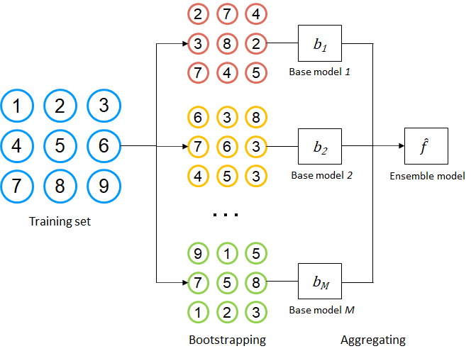It is worth noting that the size of the subsets may be smaller ( $N_s<N$ ) if the training set is large. Then, the base models are trained with these $M$ subsets. The final prediction is obtained by majority voting or simple averaging. In the case of regression, the average of all the predictions is taken as the final prediction. Figure 2 shows how bootstrapping is used to build a bagging model. As shown in the figure, an instance may appear more than one time in the subset due to sampling with replacement. For example, instance 2 and 7 appear twice in subset 1. The $M$ base models are trained on the bootstrap samples, and their predictions are aggregated by averaging or voting. Final prediction is given as follows.

$c = \arg\max_c p(c|\mathbf{x})$

where $p(c|\mathbf{x})=\sum_{m=1}^{M}w_m p_m(c|\mathbf{x})$ and $w_m=\frac{1}{M}$

Note that bagging is a method that is independent of any machine learning algorithm. In other words, we can use any algorithm to build the $M$ base models. The bagging algorithm is given as follows.

Figure 2. The bootstrap samples are used to build the base models which are then aggregated to produce the final prediction.

For  to 
   Randomly sample training subset  from  (Bootstrapping)
   Train a base model  using

Bagging exploits many base models to outperform a single model and those base models are built by training on overlapping subsets. This has the effect of reducing the variance while retaining the bias. Let us see why variance error can be reduced with bagging. The bias-variance decomposition shows that the prediction can be decomposed into bias, variance and irreducible errors where the variance error is defined as follows:

$\texttt{var} = E[(E[\hat{f}(\mathbf{x})] - \hat{f}(\mathbf{x}))^2]$

From the above, we can see that variance error will be large if the outputs of the predictive models are far away from the expected predicted value. The final prediction of a bagging model which consists of $M$ base models is defined as follows:

$\hat{f}(\mathbf{x}) = \frac{1}{M} \sum_{m=1}^M \hat{f}_m(\mathbf{x})$

Since the final prediction is the average predicted value of $M$ base models and if the number of base models is large ( $M \rightarrow \infty$ ), then the output of the bagging model will be close to the expected predicted value ( $\hat{f}(\mathbf{x}) \sim E[\hat{f}(\mathbf{x})])$ ) which in turn reduces the variance error. It is worth noting that a good reduction of variance error can be achieved if the base models are uncorrelated (diverse base models) or in other words, the base models make different errors. However, in practice, the base models could be correlated due to the generated training subsets are not significantly different. Hence, the base models will make the same errors and the variance error is not reduced.

Another advantage of bagging is that it provides an estimate of the test error without performing cross validation or holding out a test set. When bootstrapping is performed, two independent sets are created whereby one set consists of instances that are chosen by sampling with replacement. The other set is all the instances that are not chosen in the sampling process which is known as out-of-bag set. Since this out-of-bag instances are not used to train the base model, the instances can be used to obtain the test error of the model. If we do the same for all base models and compute their test errors, we obtain an estimate of the test error of the ensemble model. Formally, let $S_m$ denotes the out-of-bag set of base model $m$ . The out-of-bag error of the model is

$\epsilon_{OOB} = \frac{1}{\lvert S_m \rvert} \sum_{(\mathbf{x},y) \in S_m} l(y,h(\mathbf{x}))$

where $l$ is a loss function such as zero-one loss. The out-of-bag error is an estimate of test error since the models were not trained on the instances. If $M$ is large enough, the out-of-bag error will stabilize and converge to the cross-validation error.

Random Forest

Random forest is an extension to the bagging which combines bagging and random feature selection to build a collection of diverse decision trees [2]. Since random forest is based on bagging, each decision tree is trained on a randomly sampled subset [3]. Thus, it has all the advantages of bagging method such as the out-of-bag error and reduction of variance. But unlike bagging, during the tree building phase, only a subset of features is considered when choosing the best split-point for each decision node. The idea is to build diverse and uncorrelated to ensure optimal variance reduction can be achieved. Due to the feature randomness, the trees will be different and make different errors which will be averaged out during aggregation.

The algorithm of random forest is given as follows. For each tree, a subset is randomly sampled using bootstrapping. When building the tree using the subset, only a subset of features is used to determine the best split-point to define the decision nodes. Specifically, $k$ features are randomly chosen out of $d$ features ( $k<d$ ). Each selected feature is evaluated to determine the best-split point and the best one is chosen to define the decision node. These steps are recursively repeated until the predefined criteria are met e.g. maximum depth of the tree, the maximum number of leaf nodes etc.

Random forest has a built-in feature importance which can be obtained from the random forest construction. For each decision node in a tree, the feature with the best split-point is chosen based on some impurity functions. The impurity function can be gini or entropy for classification and sum of squared error for regression. The feature with the highest decrease of impurity is chosen for the decision node. The feature importance can be calculated as the average of impurity decrease over all decision trees in the ensemble random forest model.

for  to :
   Randomly sample training subset  from 
   Build decision tree  by repeating the following steps for each
   decision node.
      Randomly choose  features from  features
      Choose the best split-point among  features
      Define the decision node using the best split-point

References

[1] L. Breiman, “Bagging predictors,” Machine Learning, vol. 24, no. 2, pp. 123–140, Aug. 1996, doi: 10.1007/BF00058655.

[2] L. Breiman, “Random Forests,” Machine Learning, vol. 45, no. 1, pp. 5–32, Oct. 2001, doi: 10.1023/A:1010933404324.

[3] T. K. Ho, “Random decision forests,” in Proceedings of 3rd International Conference on Document Analysis and Recognition, Aug. 1995, vol. 1, pp. 278–282 vol.1. doi: 10.1109/ICDAR.1995.598994.