Ensemble Learning – Halim Noor

Introduction

Given a problem, the usual approach to solving the problem is to build several predictive models using different machine learning algorithms. When building the predictive models, we carefully choose the parameters of the models using the validation set and then evaluate and compare their performance on the test set to determine the best model. This is due to the fact that there is no single algorithm that will always give us the best model for every problem. Building an optimal predictive model with finite data is a challenging task. Machine learning algorithms come with different sets of assumptions that induce certain models. If the assumption about the data is wrong, it leads to underfitting and high bias error.

One can fine-tune the parameters to get a model with the highest validation accuracy. But finding the optimal parameters is an arduous task. In many cases, even after considerable fine-tuning, the model is still not good enough and fails on certain instances. Furthermore, in some applications such as medical and healthcare, datasets are not easy to obtain and the number of instances is typically limited. This further exacerbates the problem and the task of developing a reliable predictive model becomes somewhat infeasible. Evidently, a single model is not sufficient and there is a need for algorithms that can combine multiple models to produce better predictive models. Ensemble learning is an approach to combining the decisions of multiple models when predicting new instances [1]. The idea is that, if a model incorrectly predicts an instance, there may be another model that is able to get it right. Essentially, we want to leverage the strength of multiple models with different characteristics such that the models induce different outcomes so that they can complement each other.

Ensemble Diversity

An ensemble model supposes to perform better than any single model, that is, it should have a lower classification or regression error. We might think that a good ensemble model can be simply obtained by combining several accurate individual models. However, model accuracy is not the only consideration when building an ensemble model. More importantly, when we are building an ensemble model, the individual models or known as base models are diverse in the sense that they are making different predictions [2]. Otherwise, there would be no performance improvement even if the ensemble model is a combination of a large number of accurate models.

Building ensemble models is not an easy task. One simple approach to ensemble learning is to train multiple base models and assign a weightage to each model to indicate its importance. But this approach normally does not work because the models are trained for the same objective. The task becomes even more challenging when the same training set is used to train the models which could make them highly correlated. Furthermore, at the same time, we need to ensure the performance of the models must not very poor. Otherwise, the ensemble model’s performance would not improve or worsen.

Ensemble diversity refers to the difference among the individual models that make up the ensemble model. Several approaches have been used to achieve the goal of generating diverse models. The first approach is to use different learning algorithms to train the base models. Different learning algorithms have different inductive biases. If a base model fails to predict certain instances, other models might get them right due to their different assumptions about the data, which improves the ensemble performance. For example, one base model may be parametric (e.g. logistic regression) and others are non-parametric models (e.g. decision tree and non-linear support vector machine).

We can also build diverse base models using the same learning algorithm but with different parameters. For example, we can build different base models by varying the kernel functions in support vector machine, the number of nearest neighbors in k-nearest neighbors the tree depth and the minimum number of instances in a leaf node in decision tree [3]. If the models are trained using optimization techniques such as gradient descent in linear regression and neural network (this algorithm is discussed in a later chapter), the initial weights, learning rate and batch size are hyperparameters that can be varied to build diverse models [4].

Another approach to building diverse base models is sampling manipulation whereby the base models are trained using different training subsets. The subsets can be created using bootstrapping [5], a sampling method with replacement whereby instances are randomly drawn from the training set. Base models that are trained with different subsets are usually diverse. This ensemble learning is known as bagging which will be discussed later. The base models can also be trained sequentially whereby for each iteration (training), instances that are incorrectly predicted are given more emphasis in training subsequent base models. This ensemble learning is known as boosting.

Combination Methods

Given a set of base models, there are numerous methods to combine the predictions of the models into a single prediction. The commonly used methods are voting, linear combination and stacking.

Voting is used to combine base models that output class labels, thus it is applicable for classification ensembles. Voting combines the classification of base models by majority voting. Each base model outputs a particular class label and the class label with the most votes is chosen as the ensemble output. The voting ensemble is defined as:

$\hat{y} = \texttt{mode}(h_1(\mathbf{x}), h_1(\mathbf{x}), ..., h_M(\mathbf{x}))$

where $h_m(\mathbf{x}) \in H$ is the set of base models.

Linear combination is used to combine real-valued outputs such as class probabilities, thus it is applicable to both classification and regression ensembles. In linear combination method, each base model is assigned a weightage which implies the importance of the model. The combined probability of class $c$ of the models is defined as:

$\hat{p}(y=c \vert \mathbf{x}) = \sum_{m=1}^{M} w_m p_m(y=c \vert \mathbf{x})$

where $w_m$ is the weightage of $m$ -th base model and $w_m \geq 0$ and $\sum_{m=1}^M w_m = 1$ . If the weights are equal $w_m = \frac{1}{M}$ , this is a simple averaging. However, in practice, the base models would have different performances, hence the base models would have different weights, and finding the optimal weights manually is difficult if not infeasible [6]. One possible way to solve for $w$ is to assess the accuracies of the base models on the validation set.

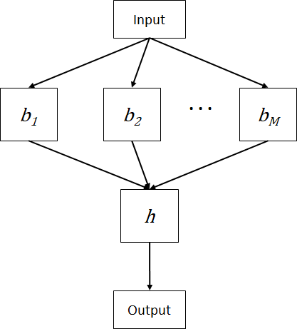
Stacking or staked generalization is a method that involves the use of machine learning algorithm to train a predictive model to combine the predictions of the base models [7]. The predictive model is referred to as the meta model. Specifically, the predictions of the base models serve as inputs to the meta model which is trained to optimally combine the predictions. In other words, the meta model learns the errors and corrects the biases of the base models. Figure 1 shows the stacking combination method whereby a meta model $h$ accepts the predictions of $M$ base models to produce the prediction. The meta model can be built using any machine learning algorithm. But in practice, logistic regression and linear regression are often used as the meta model for classification and regression problems respectively.

The training is done in two phases. First, the training set is divided into two subsets, one is for training the base models and the other one is used to train the meta model. Using the first subset, the base models are trained and the base models should be as different as possible so that they will make different errors. The second training phase uses the second subset to train the meta model. The second subset is fed to the base model to produce a set of predictions which will be used as the training input for the meta model. Then, the ensemble stacking model is evaluated on the test set by feeding the data to the base models, collecting the predictions of the base models and feeding the predictions to the meta model to get the final predictions.

Figure 1. The meta model combines the predictions of the base models.

Bagging

Bagging, short for bootstrapping aggregating, is a method to build a set of diverse base models by training them on different training subsets [8]. As the name implies, the training subsets are created by bootstrapping. Bootstrapping is a sampling method with replacement whereby instances are randomly drawn from the training set. When sampling is performed with replacement, each subset is independent of other subsets. Also, it allows some instances to appear more than once in the subsets and others may not appear at all. Thus, the subsets are different from one another, although they are drawn from the same training set. Building $M$ base models, we need $M$ subsets. For each subset, given a training set of size $N$ , we randomly draw $N_s$ instances from the training set with replacement. It is worth noting that the size of the subsets may be smaller ( $N_s<N$ ) if the training set is large. Then, the base models are trained with these $M$ subsets. The final prediction is obtained by majority voting or simple averaging. In the case of regression, the average of all the predictions is taken as the final prediction. Figure 2 shows how bootstrapping is used to build a bagging model. As shown in the figure, an instance may appear more than one time in the subset due to sampling with replacement. For example, instance 2 and 7 appear twice in subset 1. The $M$ base models are trained on the bootstrap samples, and their predictions are aggregated by averaging or voting. Final prediction is given as follows.

$c = \arg\max_c p(c|\mathbf{x})$

where $p(c|\mathbf{x})=\sum_{m=1}^{M}w_m p_m(c|\mathbf{x})$ and $w_m=\frac{1}{M}$

Note that bagging is a method that is independent of any machine learning algorithm. In other words, we can use any algorithm to build the $M$ base models. The bagging algorithm is given as follows.

Figure 2. The bootstrap samples are used to build the base models which are then aggregated to produce the final prediction.

For  to 
   Randomly sample training subset  from  (Bootstrapping)
   Train a base model  using

Bagging exploits many base models to outperform a single model and those base models are built by training on overlapping subsets. This has the effect of reducing the variance while retaining the bias. Let us see why variance error can be reduced with bagging. The bias-variance decomposition shows that the prediction can be decomposed into bias, variance and irreducible errors where the variance error is defined as follows:

$\texttt{var} = E[(E[\hat{f}(\mathbf{x})] - \hat{f}(\mathbf{x}))^2]$

From the above, we can see that variance error will be large if the outputs of the predictive models are far away from the expected predicted value. The final prediction of a bagging model which consists of $M$ base models is defined as follows:

$\hat{f}(\mathbf{x}) = \frac{1}{M} \sum_{m=1}^M \hat{f}_m(\mathbf{x})$

Since the final prediction is the average predicted value of $M$ base models and if the number of base models is large ( $M \rightarrow \infty$ ), then the output of the bagging model will be close to the expected predicted value ( $\hat{f}(\mathbf{x}) \sim E[\hat{f}(\mathbf{x})])$ ) which in turn reduces the variance error. It is worth noting that a good reduction of variance error can be achieved if the base models are uncorrelated (diverse base models) or in other words, the base models make different errors. However, in practice, the base models could be correlated due to the generated training subsets are not significantly different. Hence, the base models will make the same errors and the variance error is not reduced.

Another advantage of bagging is that it provides an estimate of the test error without performing cross validation or holding out a test set. When bootstrapping is performed, two independent sets are created whereby one set consists of instances that are chosen by sampling with replacement. The other set is all the instances that are not chosen in the sampling process which is known as out-of-bag set. Since this out-of-bag instances are not used to train the base model, the instances can be used to obtain the test error of the model. If we do the same for all base models and compute their test errors, we obtain an estimate of the test error of the ensemble model. Formally, let $S_m$ denotes the out-of-bag set of base model $m$ . The out-of-bag error of the model is

$\epsilon_{OOB} = \frac{1}{\lvert S_m \rvert} \sum_{(\mathbf{x},y) \in S_m} l(y,h(\mathbf{x}))$

where $l$ is a loss function such as zero-one loss. The out-of-bag error is an estimate of test error since the models were not trained on the instances. If $M$ is large enough, the out-of-bag error will stabilize and converge to the cross-validation error.

Random Forest

Random forest is an extension to the bagging which combines bagging and random feature selection to build a collection of diverse decision trees [9]. Since random forest is based on bagging, each decision tree is trained on a randomly sampled subset [10]. Thus, it has all the advantages of bagging method such as the out-of-bag error and reduction of variance. But unlike bagging, during the tree building phase, only a subset of features is considered when choosing the best split-point for each decision node. The idea is to build diverse and uncorrelated to ensure optimal variance reduction can be achieved. Due to the feature randomness, the trees will be different and make different errors which will be averaged out during aggregation.

The algorithm of random forest is given as follows. For each tree, a subset is randomly sampled using bootstrapping. When building the tree using the subset, only a subset of features is used to determine the best split-point to define the decision nodes. Specifically, $k$ features are randomly chosen out of $d$ features ( $k<d$ ). Each selected feature is evaluated to determine the best-split point and the best one is chosen to define the decision node. These steps are recursively repeated until the predefined criteria are met e.g. maximum depth of the tree, the maximum number of leaf nodes etc.

Random forest has a built-in feature importance which can be obtained from the random forest construction. For each decision node in a tree, the feature with the best split-point is chosen based on some impurity functions. The impurity function can be gini or entropy for classification and sum of squared error for regression. The feature with the highest decrease of impurity is chosen for the decision node. The feature importance can be calculated as the average of impurity decrease over all decision trees in the ensemble random forest model.

for  to :
   Randomly sample training subset  from 
   Build decision tree  by repeating the following steps for each
   decision node.
      Randomly choose  features from  features
      Choose the best split-point among  features
      Define the decision node using the best split-point

Boosting

Boosting is an ensemble learning algorithm that combines many weak base models to produce a strong model. A weak model is a model that performs slightly better than random guessing. Thus, a weak model has an error rate that is slightly below 50%. The model could be any machine learning model such as a decision tree with a single split which is also known as decision stump. Unlike bagging models which consist of independent base models, boosting method sequentially builds the base models in which the models are trained based on the predictions of the previous models. We describe boosting in general first. The following sections present two popular boosting algorithms, adaptive boosting and gradient boosting.

Generally, a boosting model takes the form

$\hat{f}(\mathbf{x})=\sum_{m=1}^{M} \alpha_m b(\mathbf{x};\gamma_m)$

where $\alpha_m$ is the weight of base model $m$ . The ensemble model is built in an iterative manner whereby at iteration $m$ , we add base model $\alpha_m b(\mathbf{x};\gamma_m)$ to the ensemble model. The final prediction is obtained by evaluating all the base models and taking the weighted sum.

The training is an iterative process whereby base models are added sequentially to the ensemble boosting model. At each iteration $m$ , the base model and its corresponding optimal weight are solved and added to the ensemble, and this process is repeated for $M$ base models.

$\hat{f}_m(\mathbf{x}) = \hat{f}_{m-1}(\mathbf{x}) + \alpha_m b(\mathbf{x};\gamma_m)$

Typically, the optimal base model of each iteration is trained by minimizing a loss function.

$\min_{\alpha_m, \gamma_m} \sum_{i=1}^{N} L(y^i, \alpha_m b(\mathbf{x};\gamma_m))$

where $L$ is the loss function such as the squared loss and negative log-likelihood.

Adaptive Boosting

Adaptive boosting, or simply AdaBoost [11] sequentially trains the base models on weighted training instances in which the weights are also sequentially modified to indicate the importance of the instances in the training process. Initially, the instances have equal weights. In the following iteration, the weights of the instances are individually updated based on the predictions of the base model. Those instances that were incorrectly predicted have their weights increased, while the instances that were correctly predicted have their weights decreased. Thus, the weights of the instances that are difficult to predict correctly will be ever-increased as iterations proceed, forcing the subsequent base models to focus on those instances.

Figure 3 illustrates shows the training process of AdaBoost using a simple training set. As shown in the figure, the number of iterations is 3, hence the training process builds three base models. Initially, equal weight is assigned to each instance and the base model is trained in the usual manner. Then, the weights of the instances are adjusted so that the misclassified instances are given more importance in the next iteration. In iteration $m=1$ , the three misclassified positive instances as indicated by the circle have their weights increased. This is shown by the size of those instances in iteration $m=2$ . The same procedure is followed for iteration $m=3$ .

Figure 3. A series of base models are trained on weighted instances that are individually updated for every iteration.

We describe the formulation of AdaBoost for binary classification. Although AdaBoost was initially introduced for binary classification, it has been extended to multi-class classification and regression. In AdaBoost, the optimal weak model is solved using the exponential loss which is defined as follows.

$L(\hat{f}) = e^{-y \hat{f}(\mathbf{x})}$

Consider a dataset ${(\mathbf{x}^1,y^1),(\mathbf{x}^2,y^2),...,(\mathbf{x}^N,y^N)}$ where each target $y^i \in {-1,+1}$ . At iteration $m$ , we solve for the optimal weak model $b(\mathbf{x})$ and the corresponding weight $\alpha_m$ which to be added to the ensemble model using the exponential loss.

$\begin{aligned} \alpha_m, b_m &= \arg \min_{\alpha,b} \sum_{i=1}^{N} e^{-y^i (\hat{f}_{m-1}(\mathbf{x}^i) + \alpha b(\mathbf{x}^i))} \\ &=\arg \min_{\alpha,b} \sum_{i=1}^{N} e^{-y^i \hat{f}_{m-1}(\mathbf{x}^i)} e^{-\alpha y^i b(\mathbf{x}^i) } \end{aligned}$

Let $w_m^i=e^{-y^i \hat{f}_{m-1}(\mathbf{x}^i)}$ . Note that the term does not depend on $\alpha$ and $b$ , but depends on the ensemble model $\hat{f}_{m-1}$ . Thus, we can assume $w_m^i$ as the weight of instance $i$ at iteration $m$ .

$\alpha_m, b_m = \arg \min_{\alpha,b} \sum_{i=1}^{N} w_m^i e^{-\alpha y^i b(\mathbf{x}^i) }$

The expression can be written based on two cases: misclassification ( $y \neq b(\mathbf{x})$ ) and correct classification ( $y = b(\mathbf{x})$ ).

$\alpha_m, b_m = \arg \min_{\alpha,b} \sum_{i \vert y = b(\mathbf{x}) } w_m^i e^{-\alpha } + \sum_{i \vert y \neq b(\mathbf{x})} w_m^i e^{\alpha }$

We can write $\sum_{i \vert y = b(\mathbf{x}) } w_m^i e^{-\alpha } = \sum_{i=1}^{N} w_m^i e^{-\alpha } - \sum_{i \vert y \neq b(\mathbf{x}) } w_m^i e^{-\alpha }$ . Therefore, the above expression can be written as follows.

$\begin{aligned} \alpha_m, b_m &= \arg \min_{\alpha,b} \sum_{i=1}^{N} w_m^i e^{-\alpha} - \sum_{i \vert y \neq b(\mathbf{x}) } w_m^i e^{-\alpha } + \sum_{i \vert y \neq b(\mathbf{x})} w_m^i e^{\alpha } \\ &= \arg \min_{\alpha,b} e^{-\alpha } \sum_{i=1}^{N} w_m^i + \sum_{i \vert y \neq b(\mathbf{x})} w_m^i (e^{\alpha} - e^{- \alpha}) \\ &= \arg \min_{\alpha,b} (e^{\alpha} - e^{- \alpha}) \sum_{i=1}^{N} w_m^i I(y \neq b(\mathbf{x}^i)) + e^{-\alpha} \sum_{i=1}^{N} w_m^i \end{aligned}$

Assuming the instance weights have been normalized such that $\sum_{i=1}^{N} w_m^i = 1$ . The normalization factor is a constant factor, hence it will not affect the minimization operation.

$\alpha_m, b_m = \arg \min_{\alpha,b} (e^{\alpha} - e^{- \alpha}) \sum_{i=1}^{N} w_m^i I(y \neq b(\mathbf{x}^i)) + e^{-\alpha}$

From the above, since $e^{\alpha} - e^{- \alpha}$ is a positive value, we see that the weak base model $b_m$ to be added is

$b_m= \arg \min \sum_{i=1}^{N} w_m^i I(y \neq b(\mathbf{x}^i))$

We can see that this is actually the weighted error of the base model. Note that the base model doesn’t have to be strong. It is sufficient that the weighted error is less than 0.5.

Now, we need to solve for $\alpha_m$ . Let’s us denote the weighted error as $\epsilon_m = \sum_{i=1}^{N} w_m^i I(y \neq b(\mathbf{x}^i))$ . We substitute $\epsilon_m$ into the expression.

$\begin{aligned} \alpha_m &= \arg \min_{\alpha,b} (e^{\alpha} - e^{- \alpha}) \epsilon_m + e^{-\alpha} \\ &= \arg \min_{\alpha,b} e^{\alpha} \epsilon_m - e^{-\alpha} \epsilon + e^{-\alpha} \end{aligned}$

We take the derivative with respect to $\alpha$ , and then divide it by $e^{-\alpha}$ .

$\begin{aligned} \frac{\partial (e^{\alpha} \epsilon_m - e^{-\alpha} \epsilon + e^{-\alpha})}{\partial \alpha} &= e^{\alpha} \epsilon_m + e^{-\alpha} \epsilon_m - e^{-\alpha} \\ &= e^{2\alpha} \epsilon_m + \epsilon_m + 1 \end{aligned}$

Setting it to zero to solve for the minimum.

$\begin{aligned} e^{2\alpha} \epsilon_m + \epsilon_m + 1 &= 0 \\ e^{2\alpha} &= \frac{1-\epsilon_m}{\epsilon_m} \\ 2\alpha &= \ln \frac{1-\epsilon_m}{\epsilon_m} \\ \alpha_m &= \frac{1}{2} \ln \frac{1-\epsilon_m}{\epsilon_m} \end{aligned}$

Therefore, the ensemble model is then updated

$\hat{f}_{m+1}(\mathbf{x}) = \hat{f}_{m}(\mathbf{x}) + \alpha_m b_m(\mathbf{x})$

Recall that $w_m^i=e^{-y^i \hat{f}_{m-1}(\mathbf{x}^i)}$ . The weights of the next iteration is

$\begin{aligned} w_{m+1}^i &= e^{-y^i \hat{f}_m(\mathbf{x}^i)} \\ &= e^{-y^i (\hat{f}_{m-1}(\mathbf{x}^i) + \alpha_m b_m(\mathbf{x}^i)) } \\ &= e^{-y^i \hat{f}_{m-1}(\mathbf{x}^i)} \cdot e^{-y^i b_m(\mathbf{x}^i) \alpha_m} \\ &= w_m^i \cdot e^{-y^i b_m(\mathbf{x}^i) \alpha_m} \end{aligned}$

We can rewrite $-y^i b_m(\mathbf{x}^i) = 2 \cdot I(y^i \neq b_m(\mathbf{x}^i)) - 1$ . Thus, the weight update becomes

$\begin{aligned} w_{m+1}^i &= w_m^i \cdot e^{(2 \cdot I(y^i \neq b_m(\mathbf{x}^i)) - 1) \alpha_m} \\ &= w_m^i \cdot e^{\alpha_m 2 \cdot I(y^i \neq b_m(\mathbf{x}^i)) - \alpha_m} \\ &= w_m^i \cdot e^{\alpha_m 2 \cdot I(y^i \neq b_m(\mathbf{x}^i))} \cdot e^{-\alpha_m} \end{aligned}$

Notice that the term $e^{-\alpha_m}$ multiplies all the weights by the same value and it will be canceled out in the normalization step. Thus, it has no effect on the weight update and can be dropped.

Putting everything together, the algorithm of AdaBoost is given below.

Initialize the instance weights  where 
for  to M
   Train a base model  using the weighted training set.
   Compute 
   if 
      Compute 
      
      Set 
   else
      return 
Return

Gradient Boosting

Gradient boosting is a generalized boosting algorithm that is based on gradient descent. Recall that gradient descent is used to approximate the function (predictive model) by minimizing the loss function. This is done by computing the gradients of the loss function with respect to the weights which are then used to update the weights. Using the same approach, we can search the same way over functions instead of the weights [12-13].

Consider a gradient boosting algorithm with $M$ steps. The algorithm begins with a random guessed function as the initial weak base model, which could be the average function as indicated by the black line in Figure 4. For each subsequent $m$ steps, we add a base model that will correct the error of its predecessor’s predictions. This is done by calculating the difference between the predictions and the true values as indicated by the blue line. The prediction error which is also known as residual, is then used as the target to train the base model and add it to the ensemble model. The reasoning behind this is that if we can approximate the residuals, we can use it to correct wherever errors it had made. This is shown in the figure on the right, the residuals have been reduced when the average function is added with the newly built base model.

Figure 4. The base model is trained on the residuals to improve the prediction.

We describe the formulation of gradient boosting for regression. Given a loss function

$L(\hat{f})=\sum_{i=1}^{N}L(y^i,\hat{f}(\mathbf{x}^i))$

where $L(y^i,\hat{f}(\mathbf{x}^i))$ is the regression loss such as squared loss function and $\hat{f}$ is the approximated function or the trained model. The aim is to minimize $L(\hat{f})$ with respect to $\hat{f}$ . Recall that in boosting, weak base models are sequentially added to produce an ensemble model. Thus, minimizing the loss function can be viewed as

$\mathrm{\hat{f}} = \arg \min L(\hat{f})$

where $\mathrm{\hat{f}} = (\hat{f}(\mathbf{x}^1),\hat{f}(\mathbf{x}^2),...,\hat{f}(\mathbf{x}^N) )$ . The optimization problem is solved using gradient descent. At step $m$ , the gradient of $L(\mathrm{\hat{f}})$ is

$g_m^i=[\frac{\partial L(y^i,\hat{f}(\mathbf{x}^i))}{\partial \hat{f}(\mathbf{x}^i)}]_{\hat{f}=\hat{f}_{m-1}}=-(y^i - \hat{f}(\mathbf{x}^i))$

We would like to reduce the residuals of the previous step. Thus the negative gradient is taken

$r_m^i= -g_m^i = (y^i-\hat{f}(\mathbf{x}^i))$

Train $b_m(\mathbf{x},\gamma_m)$ using the ${(\mathbf{x}^1,r^1),(\mathbf{x}^2,r^2),...,(\mathbf{x}^N,r^N)}$ .

$\gamma_m = \arg \min \sum_{i=1}^N (r_m^i - b(\mathbf{x}^i, \gamma))^2$

Finally, add $b_m$ to the ensemble model.

$\hat{f}_m = \hat{f}_{m-1} + \alpha b_m$

where $\alpha$ is a constant value typically in the range of 0 and 1.

In practice, the base model is implemented a decision tree with a limited depth e.g. maximum depth of 3. Gradient boosting can be used for both regression and classification. For classification, the log loss (binary cross entropy) is used as the loss function. Putting everything together, the algorithm of gradient boosting is given below.

for  to 
   Compute the gradient residual 
   Train a base model which minimize 
   Update 
Return

References

[1] D. Opitz and R. Maclin, “Popular Ensemble Methods: An Empirical Study,” Journal of Artificial Intelligence Research, vol. 11, pp. 169–198, Aug. 1999, doi: 10.1613/jair.614.

[2] P. Sollich and A. Krogh, “Learning with Ensembles: How over-Fitting Can Be Useful,” in Proceedings of the 8th International Conference on Neural Information Processing Systems, Cambridge, MA, USA, 1995, pp. 190–196.

[3] F. T. Liu, K. M. Ting, and W. Fan, “Maximizing Tree Diversity by Building Complete-Random Decision Trees,” in Advances in Knowledge Discovery and Data Mining, Berlin, Heidelberg, 2005, pp. 605–610. doi: 10.1007/11430919_70.

[4] J. F. Kolen and J. B. Pollack, “Back propagation is sensitive to initial conditions,” in Proceedings of the 1990 conference on Advances in neural information processing systems 3, San Francisco, CA, USA, Oct. 1990, pp. 860–867.

[5] B. Efron and R. J. Tibshirani, An introduction to the bootstrap. CRC press, 1994.

[6] Z.-H. Zhou, Ensemble Methods: Foundations and Algorithms, 1st ed. Chapman & Hall/CRC, 2012.

[7] D. H. Wolpert, “Stacked generalization,” Neural Networks, vol. 5, no. 2, pp. 241–259, Jan. 1992, doi: 10.1016/S0893-6080(05)80023-1.

[8] L. Breiman, “Bagging predictors,” Machine Learning, vol. 24, no. 2, pp. 123–140, Aug. 1996, doi: 10.1007/BF00058655.

[9] L. Breiman, “Random Forests,” Machine Learning, vol. 45, no. 1, pp. 5–32, Oct. 2001, doi: 10.1023/A:1010933404324.

[10] T. K. Ho, “Random decision forests,” in Proceedings of 3rd International Conference on Document Analysis and Recognition, Aug. 1995, vol. 1, pp. 278–282 vol.1. doi: 10.1109/ICDAR.1995.598994.

[11] Y. Freund and R. E. Schapire, “A Decision-Theoretic Generalization of On-Line Learning and an Application to Boosting,” Journal of Computer and System Sciences, vol. 55, no. 1, pp. 119–139, Aug. 1997, doi: 10.1006/jcss.1997.1504.

[12] J. H. Friedman, “Greedy Function Approximation: A Gradient Boosting Machine,” The Annals of Statistics, vol. 29, no. 5, pp. 1189–1232, 2001.

[13] J. H. Friedman, “Stochastic gradient boosting,” Computational Statistics & Data Analysis, vol. 38, no. 4, pp. 367–378, Feb. 2002, doi: 10.1016/S0167-9473(01)00065-2.