Exchangeability and Bias-Variance Decomposition

Exchangeability

Machine learning algorithms cannot understand or do not model the cause and effect relationships which is necessary to explain why something happens. In real-world scenarios, there are causal relationships between actions and consequences such as when a patient has a fever and headache because of dengue, the dengue is the cause, and the effects are fever and headache. So, how do machine learning models able to predict the output given an input? A machine learning model gets its predictive power by eliminating the differences in data, ignoring the outliers, reducing the errors and finding the mapping between the inputs features and the output. Since the machine learning algorithms are not able to attribute predictions to causes, they rely on a concept called exchangeability to ensure we can build useful predictive models.

What is exchangeability? When we train a predictive model for a particular problem, we use a dataset that contains samples of the whole population. We assume the samples in the dataset are sufficiently representative. Specifically, the size of the dataset should not only be large enough, but the data should also be representative of the actual environment. Therefore, the predictive models that we build using the dataset can be applied to predict unknown new data. This assumption is made on the basis that the unknown future data is exchangeable with the training data. This concept of data exchangeability assumes that the training data and test data are independent and identically distributed or known as IID.

The assumption that data are independent and identically distributed is essential in machine learning. Independent means each instance is unrelated to every other instance in the dataset. Identically distributed means the instances are sampled from the same probability distribution. Consider a dataset on hospital patients. The dataset is independent and identically distributed if each patient’s data is independent or is unrelated to other patients’ data and they have the same probability distribution, or in other words, the law that generates the data is the same from one patient to another.

Bias-Variance Decomposition

The main goal of machine learning is to find a function that is a good approximation $\hat{f}(\mathbf{x};D_{tr})$ of the true function based on the training set $D_{tr}$ . In a regression setting, a good function is learned by quantifying the difference between the response variable $y$ and the prediction $\hat{y}=\hat{f}(\mathbf{x};D_{tr})$ using the squared loss. Specifically, we want the squared loss to be minimal for both $D_{tr}={(x^1,y^1), (x^2,y^2), ..., (x^N,y^N)}$ and data points not in the training set. Ideally, we want the learned function to be perfect (minimal prediction error), however, such a function is not possible due to the limitation of the machine learning algorithm and noise in the data.

The prediction error can be decomposed into irreducible error and reducible error. The irreducible error is due to the fact that the data that we have are not able to completely describe the target being predicted. There are other features not within the dataset that have some effect on the target. Consider a problem of predicting the sales of a food truck given its location and number of tourists. The features might be able to give a prediction, but they will not explain everything because there are other factors that affect the sales such as the weather, the raw material shortage and other issues intrinsic to the problems that are being modeled.

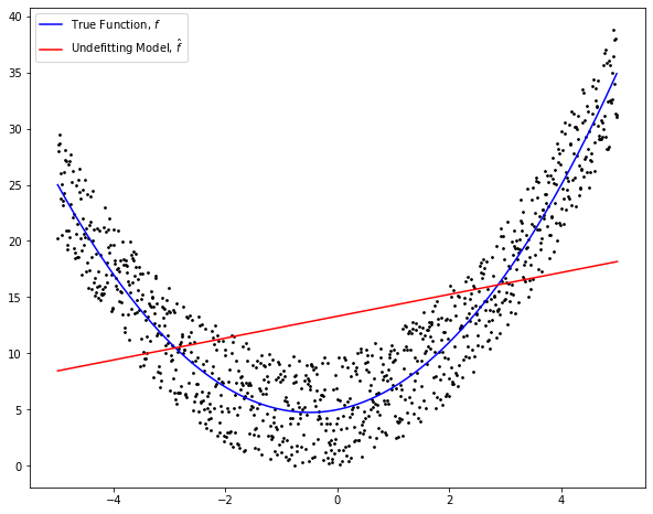
The reducible error is the error that is associated with the predictive model which can be decomposed into bias and variance errors. Bias error refers to the amount of difference between the target and the prediction of the model. Every machine learning algorithm comes with a set of assumptions that forms the inductive bias of the predictive model. For example, the linear regression algorithm assumes a linear relationship between the features and the target, hence the model is described in the form of a linear equation. However, if the assumption does not hold, it may lead to a high inductive bias error. We call this underfitting model. Figure 1 illustrates a linear model indicated by the red line which does not approximate well the true function indicated by the blue curve.

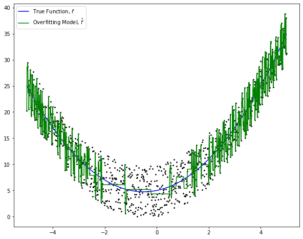
Figure 1. A predictive model with inductive bias due to its simplistic assumption about the data.

On the other hand, some powerful machine learning algorithms such as decision tree and support vector machine make strong assumptions about the data. The algorithms will be discussed in the later chapters. Due to their strong learning ability, the algorithms can learn every variation including the randomness in the data. Thus, the predictive models have low inductive bias error, but high variance error whereby the models are sensitive to small fluctuations in the data. Variance error also reflects the variability in the model prediction. It shows the inconsistency of the model across different datasets. This phenomenon is known as overfitting whereby the models do not generalize well on new data. Figure 2 illustrates an overfitting model in which the model fits the data very closely as indicated by the green line.

Figure 2. An overfitting predictive model learns the variation of the data very closely.

Suppose the data is generated by a function (model) $y=f(\mathbf{x}) + \epsilon$ , with $E(\epsilon)=0$ and $\texttt{var}(\epsilon) = \sigma^2$ . The derivation of the bias-variance decomposition of the squared loss is as follows.

$\begin{aligned} E[(y-\hat{f})^2] &= E[(f+\epsilon-\hat{f})^2] \\ &= E[(f - E(\hat{f}) + E(\hat{f}) -\hat{f} + \epsilon)^2] \end{aligned}$

Using $(a+b+c)^2 = a^2 + b^2+c^2 + 2ab+2ac+2bc$ and assuming $a=f - E(\hat{f})$ , $b=E(\hat{f}) -\hat{f}$ and $c=\epsilon$ , we can expand the equation as follows:

$\begin{aligned} E[(y-\hat{f})^2] = & E[(f - E[\hat{f}])^2] + E[(E[\hat{f}] -\hat{f})^2] + E[\epsilon^2] \\ & +2E[\epsilon(E[\hat{f}] -\hat{f})] + 2E[\epsilon(f - E[\hat{f}])] \\ &+ 2E[(f - E[\hat{f}])(E[\hat{f}] -\hat{f})] \end{aligned}$

$\begin{aligned} E[(y-\hat{f})^2] = & (f - E[\hat{f}])^2 + E[(E[\hat{f}] -\hat{f})^2] + E[\epsilon^2] \\ & + 2E[\epsilon](E[\hat{f}] -\hat{f}) + 2E[\epsilon]E[(f - E[\hat{f}])] \\ & + 2E[E[\hat{f}] -\hat{f}](f - E[\hat{f}]) \end{aligned}$

We know that $E[E[\hat{f}] -\hat{f}]=E[\hat{f}] - E[\hat{f}] = 0$ . Thus, the equation is reduced to

$\begin{aligned} E[(y-\hat{f})^2] &= (f - E[\hat{f}])^2 + E[(E[\hat{f}] -\hat{f})^2] + E[\epsilon^2] \\ &= (f - E[\hat{f}])^2 + E[(E[\hat{f}] -\hat{f})^2] + \texttt{var}(\epsilon) \\ &= \texttt{bias}(\hat{f})^2 + \texttt{var}(\hat{f}) + \sigma^2 \end{aligned}$

where $\texttt{bias}$ and $\texttt{var}$ are the bias and variance errors and $\sigma^2$ is the irreducible error.

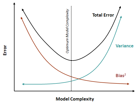
Ideally, we want to build a model that has both small bias and variance errors, a model that learns the patterns of the data accurately and generalizes well to unseen data. However, in practice, we must make a trade-off between increasing the model complexity to capture the variation in the data and simplifying the model to avoid overfitting as shown in Figure 3. Simple machine learning algorithms such as linear regression make less assumption about the data. Thus, the algorithm often produces predictive models with high bias error but they are consistent across datasets and are not sensitive to changes in the data. More complex machine learning algorithms such as decision tree and support vector machine have more parameters that can be manipulated to learn the underlying structure of the data. Thus, the algorithms may produce models with low bias error. But, the models tend to have higher variance and there is a risk of overfitting the data. Hence, we need to find the optimal balance between bias and variance.