Gradient Descent – Halim Noor

Gradient descent is an optimization algorithm for finding a local minimum of a differentiable function. The algorithm iteratively updates the parameters of the function by computing the gradient of the function. Consider a differentiable function, $f(x)=x^2-10x$ as shown in Figure 1. We know that the function is minimum when $x=5$ . Assuming that $x=12$ , to get to the minimum, we need to move to the “left”. Specifically, we need to update $x$ by subtracting a value from it. To determine the value that we need to subtract from $x$ , we compute the gradient at $x=12$ which is the slope of the tangent line at the given point. In other words, the gradient is the rate of change of the function at a given point.

Figure 1. The gradient is the slope of the tangent line at a given point.

Given a function, the gradient is computed by taking the derivative of the function with respect to its parameter.

$\frac{\partial f}{\partial x} = 2x - 10$

Then, the parameter is updated iteratively until optimal solution is obtained as follows:

Repeat until converge: $x := x - \alpha \frac{\partial f}{\partial x}$

where $0 \leq \alpha \leq 1$ is the step size or learning rate. $\alpha$ controls the amount of the update to be applied to the parameter $x$ . A small $\alpha$ corresponds to a little step which means the optimization will take longer to complete while a large $\alpha$ may cause the gradient descent to overshoot (miss the minimum) and fail to converge.

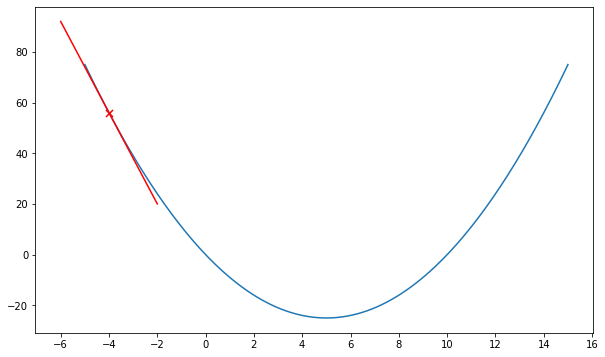
Let’s analyze the parameter update equation. Consider $x=12$ as shown in Figure 1. For now, assuming $\alpha = 1$ . We know that $\frac{\partial f}{\partial x}>0$ (positive value). Based on the update equation, $x$ will be reduced by the value of $\frac{\partial f}{\partial x}$ .

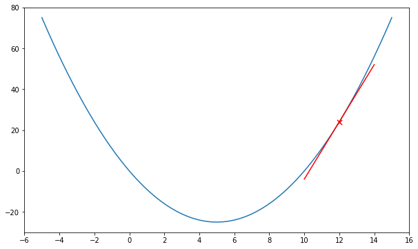
If $x$ is to the left of the minimum as shown in Figure 2. We know $\frac{\partial f}{\partial x}<0$ (negative value). Based on the update equation, $x$ will be increased by the value of $\frac{\partial f}{\partial x}$ .