k-Means Clustering

Introduction

In many cases, we are given a dataset but the instances have no labels associated with it. Specifically, we are given only $\mathbf{x}^i$ and not the labels $y^i$ . Thus, we do not know how many labels are there in the data, and which $\mathbf{x}^i$ comes from which $y^i$ . This dataset is known as unlabeled dataset $D={\mathbf{x}^1, \mathbf{x}^2,...,\mathbf{x}^N}$ . Since the labels are not known, we need to estimate the labels. Then, given the labels, we estimate the labels of the instances based on certain assumptions as shown in Figure 1. This problem is known as clustering.

Figure 1. Clustering is partitioning the instances into a number of groups (clusters) such that instances belonging to a group are close to each other.

Suppose we have a dataset consisting of $N$ instances. We want to partition the instances into $K$ clusters. We can view a cluster as a group of data points that are close to each other which means the distances between the data points within the cluster is smaller than the distances between the data points and the data points outside the cluster. Thus, in k-means, the clusters are represented by the center of clusters, also known as the centroid. The k-means clustering process can be divided into two repeating steps: cluster assignment and centroid update. The assignment step assigns data points to one of the $K$ clusters based on the distance between the data points and the centroids. Let $\mathbf{\mu}_k$ denote the centroid $k$ . Data point $\mathbf{x}^i$ is assigned to cluster $\mathbf{\mu}_k$ whereby the distance between the data point and the centroid is minimum.

$r^i = \arg\min_k \lVert \mathbf{x}^i - \mathbf{\mu}_k \rVert^2$

where $r^i$ is the index of cluster $k={1,2,...,K}$ to which $\mathbf{x}^i$ is assigned to and $\lVert \mathbf{x}^i - \mathbf{\mu}_k \rVert^2$ is the euclidean distance.

After the assignment step, each centroid is updated by calculating the mean of the data points that are assigned to it. Let $N_k$ denote the number of data points that are assigned to cluster $k$ . The centroid update is given as follows:

$\mathbf{\mu}_k = \frac{1}{N_k} \sum_{i: r^i=k} \mathbf{x}^i$

The goal is to find the assignment of the data points such that the distances between the data points of the clusters and their centroids are minimum. Thus, the two steps are repeated to minimize the following objective function.

$(r^1,...,r^N, \mathbf{\mu}, ...,\mathbf{\mu}^K) = \arg \min_{(r^1,...,r^N, \mathbf{\mu}^1, ...,\mathbf{\mu}^K)} \sum_{i=1}^N \lVert \mathbf{x}^i - \mathbf{\mu}_{r^i} \rVert^2$

Algorithm

k-means algorithm is given below. We begin by specifying the number of clusters $K$ . Each centroid is randomly initialized. In the next section, we will discuss an improved initialization method for the centroids. Then, repeatedly assign each data point to its nearest centroid and update each centroid by calculating the mean of all data points assigned to it. The algorithm is terminated when the assignments no longer change. Figure 2 illustrates the k-means clustering process.

initialize 
repeat until converged
   assignemnt: .
   update: .

Figure 2. k-means steps are performed repeatedly until converged.

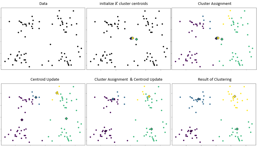
Numerical Example

Consider the following set of data points.

$\mathbf{x}=\begin{bmatrix} 4&3\\5&4\\1&1\\2&1 \end{bmatrix}$

Suppose $k=2$ . Initialize the centroids.

$\mathbf{\mu}_k=\begin{bmatrix} 1&1 \\2&1 \end{bmatrix}$

For each data point, calculate its distance to the centroids.

For example, the distance between $x^1$ and $\mu_1$ and $\mu_2$ are

$d_1^1=\sqrt{(4-1)^2+(3-1)^2}=3.61$

$d_2^1=\sqrt{(4-2)^2+(3-1)^2}=2.83$

$d_1=\begin{bmatrix} 3.61\\5\\0\\1 \end{bmatrix}$

$d_2=\begin{bmatrix} 2.83\\4.24\\1\\0 \end{bmatrix}$

For each data point, assign it to the closest centroid.

$r=\begin{bmatrix} 2\\2\\1\\2 \end{bmatrix}$

Update the centroids.

$\mu_1=(1,1)$

$\mu_2=(\frac{4+5+2}{3},\frac{3+4+1}{3}) = (\frac{11}{3},\frac{8}{3})$

Repeat until the assignment is no longer change.

k-Means++

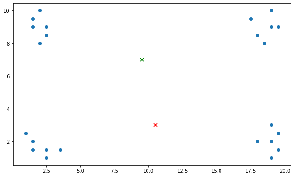
Random initialization could lead to inconsistency and sub-optimal clustering. Consider a set of data points as shown in Figure 3. Assuming the number of clusters is 2 and the centroids are initialized randomly and happen to be at the location indicated by “x” marker in green and red colors. The data points at the top region are closer to the green marker while the data points at the bottom region are closer to the red marker. The k-means algorithm will converge with the data points at the bottom region clustered together and the data points at the top region forming the second cluster. This is a sub-optimal clustering because the distance between the data points on the left and right is larger than the distance of the data points from the top to the bottom.

k-means++ is an initialization method for k-means clustering algorithm. Rather than just randomly initialize the centroids, k-means++ randomly chooses one of the data points to be the first centroid. Then, the subsequent centroids are chosen from the remaining data points with the probability proportional to the distance of the data points to the previously chosen centroid. As a result, the centroids will be far away from each other. The algorithm of k-means++ is given as follows:

Randomly pick one data point as the first centroid .
for  to  do
   Compute the distance of each data point from .
      .
   Compute the probability for each data point.
      
   Choose one data point with the largest probability as .

Choosing the value of k

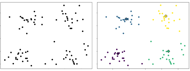
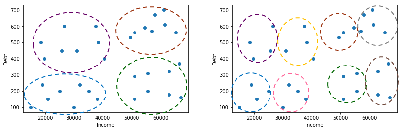
As we discussed above, the number of clusters affects the clustering result. Thus, it is important to carefully choose the value of k. Unfortunately, there is no standard method to choose the value of k. It is common for the value of k to be chosen manually through visualization or based on domain knowledge. Typically, the value of k is estimated based on some later or downstream purpose. For example, consider a clustering problem in banking as shown in Figure 3(right). The features are Income and Debt. The data points can be grouped into four clusters. The clusters at the lower regions may represent customers with low debt, one with low income indicated by the blue oval and the second cluster with high income indicated by the green oval. The clusters at the top region represents customer with high debt and low income (purple oval) and high income (brown oval). Instead of four clusters, the data points can be grouped into eight clusters in which the clusters represent customers with low debt and high debt, but with different income scales as shown in Figure 3(left).

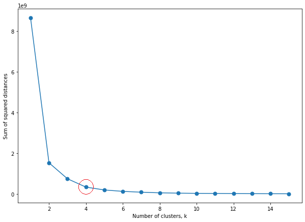
Figure 3. The number of clusters is defined based on a downstream purpose.

Another way of defining the number of clusters is to determine the value based on the objective function. The objective function which is the sum of squared distances between the data points and their centroids indicates the compactness of the clusters. As the value of k increases, the sum of squared distances decreases because each cluster will have fewer data points and the data points will be closer to their clusters. However, at some point, the rate of decrease of the sum of squared distances will start to decline due to overfitting. The value of k at which the decrease rate starts to decline is known as the elbow. Figure 4 shows a plot of sum of squared distances againts different values of k. A sharp decrease in sum of squared distances can be observed for the number of clusters equal to 2 to 4. Also, it is observed that the sum of squared distances starts to stagnant for the following number of clusters. Thus, the value of k is chosen to be 4.