k-Nearest Neighbors – Halim Noor

Introduction

Machine learning algorithms can be categorized into parametric and non-parametric. Parametric model refers to a model with a specific functional form that is defined by a fixed number of parameters. The machine learning algorithms that we have seen in the previous chapters, linear regression and logistic regression are examples of parametric models whereby the models are in linear form. The advantages of parametric models are simple, fast to compute and require less training data due to its strong assumption about the data. However, the assumption may not hold which may lead to large error. Non-parametric model refers to models that their number of parameters grows with the amount of training data. Unlike parametric models, non-parametric models do not assume any specific functional form. The models are not making strong assumptions about the data; hence they are more flexible and powerful. But the complexity of the models grows with the size of the training set and can be computationally infeasible for very large datasets.

k-nearest neighbors is a non-parametric algorithm that can be used for classification and regression. The algorithm assumes that instances that belong to the same class tend to be close to each other. In other words, data points are not randomly distributed across the feature space, but rather, spatially clustered as shown in Figure 1. As shown in Figure 1, the data points (instances) belong to three classes, with the label $y$ coded as 0 for BLUE, 1 for ORANGE and 2 for GREEN. Data points belonging to BLUE are distributed in the upper left region of the feature space. The GREEN and ORANGE data points are distributed in the lower right of the feature space with the GREEN data points occupying the upper part of the region while ORANGE data points occupying the lower part of the region.

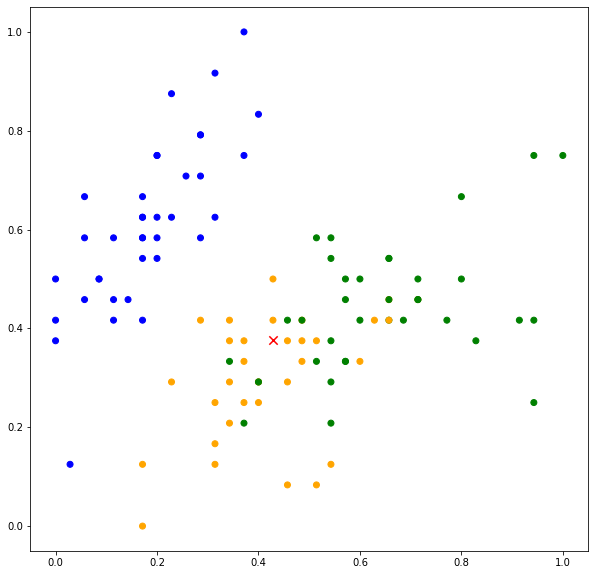
Figure 1. Data points appear in clusters of three classes.

On the basis of this assumption, if we are given a new data point, the label of the data point can be determined based on the neighboring data points. Consider a new data point indicated by “x” marker in red color. Based on its location, we can somehow deduce that the data point belongs to ORANGE. This is because there are more ORANGE data points neighboring the new data point.

Specifically, k-nearest neighbors algorithm uses $k$ data points in the training set that are nearest to the test input (new data point) to decide the label of the test point. Let $\acute{x}$ denotes a test input and $S_n \subseteq{D_{tr}}$ denotes the set of $k$ nearest neighbors of $\acute{x}$ . The $k$ nearest neighbors are data points with distances smaller than distances of other data points.

Let input-output pairs in the training set but not in $S_n$ be $\forall(x,y) \in{D_{tr}} \setminus S_n$ . The distance of nearest neighbors, $x_n$ is

$\max(\text{dist}(x_n,\acute{x})) \leq \text{dist}(x,\acute{x})$ .

The prediction of k-nearest neighbor classifier is defined as follows:

$p(y=c|\acute{x},k)=\frac{1}{k} \sum_{(x_n,y_n) \in{S_n}} I(y_n=c)$

where $I(e)=\begin{cases} 1 & \text{if }e \text{ is true} \\ 0 & \text{if }e \text{ is false} \end{cases}$

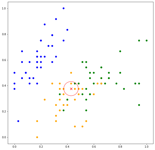
k-nearest neighbors is an example of memory-based or instance-based learning. The predictive model is the set of training instances and $k$ is the parameter of the algorithm (needs to be set), which determines the number of neighbors that will be considered in the prediction. Consider $k=3$ , the neighbors consist of two data points belonging to ORANGE and one data point belonging to GREEN as shown in Figure 2(top). 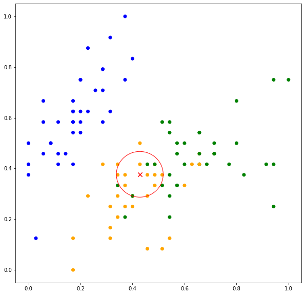The predicted values are $p(y=0, \mathbf{x})=0.0$ , $p(y=1, \mathbf{x})=0.667$ , $p(y=2, \mathbf{x})=0.333$ .

Thus, the test point is classified as ORANGE. Now when $k=10$ , more neighboring data points are considered in the classification. As can be seen in Figure 2(bottom), out of ten data points, eight data points belong to ORANGE while two belong to GREEN. The predicted values are $p(y=0, \mathbf{x})=0.0$ , $p(y=1, \mathbf{x})=0.8$ , $p(y=2, \mathbf{x})=0.2$ .

Note the increase in probability estimate of $p(y=1,\mathbf{x})$ . In general, the prediction is more susceptible to noise when the value of $k$ is small. A large value of $k$ reduces the effect of noise on the prediction but is more computationally expensive. However, the optimal value of $k$ depends on the data and should be empirically selected using the validation set. Furthermore, $k$ must be a positive and non-zero value. It is also advisable to choose an odd value to avoid equal scores for binary classification.

Distance Functions

k-nearest neighbor algorithm relies on a distance function to determine the neighbors of the test input. The most commonly used distance function is the Euclidean distance. Euclidean distance measures the straight line distance between two data points. The distance function is defined as follows:

$\text{dist}(x_n,\acute{x}) = \sqrt{\sum_{i=1}^{\lvert S_n \rvert} (x_n^i - \acute{x^i})^2$

Alternative to Euclidean distance is the Manhattan distance. Manhattan distance is the distance between two points measured at right angle along the vertical and horizontal axes.

$\text{dist}(x_n,\acute{x}) = \sum_{i=1}^{\lvert S_n \rvert} (\lvert x_n^i - \acute{x^i} }\rvert)$

Hamming distance is used for categorical variables whereby the distance is measured as the number of different symbols between the two instances. For example, the Hamming distance between two instances consists of three features as follows is 2.

$\mathbf{x}^1 = (\text{Yes}, \text{Pass}, \text{High})$

$\mathbf{x}^2 = (\text{No}, \text{Fail}, \text{High})$

References

[1] T. Cover and P. Hart, “Nearest neighbor pattern classification,” IEEE Transactions on Information Theory, vol. 13, no. 1, pp. 21–27, Jan. 1967, doi: 10.1109/TIT.1967.1053964.