Linear Discriminant Analysis

Introduction

Principal component analysis projects the data in the directions of maximum variance. However, in some cases, maximizing the variance of the data may not achieve highly discriminative features. Fisher’s Linear discriminant analysis (LDA) is also a projection-based method that seeks to find a vector that defines the projection direction of the data [1]. Unlike principal component analysis which maximizes the variance of the data [2], linear discriminant analysis uses the labels of the data and projects the data in the direction that maximizes the separation of the classes as shown in Figure 1.

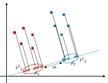
Figure 1. Projection direction maximizes the maximum class separation.

How do we find the projection that maximizes the class separation of the data? LDA states that maximum separation is achieved when the distance between the two clusters is maximum (or far away from each other). We consider the classification of two classes first, then generalize to more than two classes.

Binary Class LDA

Let $\tilde{\mu}_1$ and $\tilde{\mu}_2$ denote the means of data after projection which belong to class RED and BLUE respectively.

$\tilde{\mu}_1=\mathbf{w}^T \mathbf{\mu_1}$

Furthermore, let $\tilde{s}^2_1$ and $\tilde{s}^2_2$ denote the scatters (variances) of data after projection which belong to class RED and BLUE respectively.

$\tilde{\mu}_2=\mathbf{w}^T \mathbf{\mu_2}$

$\tilde{s}^2_1 = \sum_{x \in c_1} (\mathbf{w}^T\mathbf{x} - \mathbf{w}^T \mathbf{\mu_1})^2$

$\tilde{s}^2_2 = \sum_{x \in c_2} (\mathbf{w}^T\mathbf{x} - \mathbf{w}^T \mathbf{\mu_2})^2$

To ensure maximum class separation, we want the means to be far away from each other and the projected data in the clusters to be close to each other. In other words, we want the mean difference $\lvert \tilde{\mu}_1 - \tilde{\mu}_2 \rvert$ to be large and the summation of the scatter $\tilde{s}^2_1 + \tilde{s}^2_2$ to be small. Therefore, the objective is to maximize

$J(\mathbf{w})=\frac{\lvert \tilde{\mu}_1-\tilde{\mu}_2 \rvert^2}{\tilde{s}^2_1 + \tilde{s}^2_2}$

The numerator can be expressed as

$\begin{aligned}\lvert \tilde{\mu}_1-\tilde{\mu}_2 \rvert^2 &= \lvert \mathbf{w}^T \mathbf{\mu_1} - \mathbf{w}^T \mathbf{\mu_2} \rvert^2 \\ &= \mathbf{w}^T(\mathbf{\mu_1} - \mathbf{\mu_2})(\mathbf{\mu_1} - \mathbf{\mu_2})^T\mathbf{w} \\ &= \mathbf{w}^Ts_B\mathbf{w} \end{aligned}$

where $s_B = (\mathbf{\mu_1} - \mathbf{\mu_2})(\mathbf{\mu_1} - \mathbf{\mu_2})^T$ is between-class scatter matrix.

The denominator can be expressed as

$\begin{aligned} \tilde{s}^2_k &= \sum_{x \in c_k} (\mathbf{w}^T\mathbf{x} - \mathbf{w}^T \mathbf{\mu_k})^2 \\ &= \sum_{x \in c_k} (\mathbf{w}^T\mathbf{x} - \mathbf{w}^T \mathbf{\mu_k})(\mathbf{w}^T\mathbf{x} - \mathbf{w}^T \mathbf{\mu_k}) \\ &= \sum_{x \in c_k} \mathbf{w}^T(\mathbf{x}-\mathbf{\mu_k})(\mathbf{x}-\mathbf{\mu_k})^T \mathbf{w} \\ &= \mathbf{w}^T \sum_{x \in c_k} (\mathbf{x}-\mathbf{\mu_k})(\mathbf{x}-\mathbf{\mu_k})^T \mathbf{w} \\ &= \mathbf{w}^T s_W \mathbf{w} \end{aligned}$

where $s_W=\sum_{x \in c_k} (\mathbf{x}-\mathbf{\mu_k})(\mathbf{x}-\mathbf{\mu_k})^T$ is within-class scatter matrix.

Therefore, the objective function is

$J(\mathbf{w})=\frac{\mathbf{w}^Ts_B\mathbf{w}}{\mathbf{w}^T s_W \mathbf{w}}$

Taking the derivative and setting it equal to zero.

$\begin{aligned} \frac{(\mathbf{w}^T s_W \mathbf{w})2s_B\mathbf{w} - (\mathbf{w}^Ts_B\mathbf{w})2s_W\mathbf{w}}{2\mathbf{w}s_W\mathbf{w}} &=0 \\ s_B\mathbf{w} - \frac{\mathbf{w}^Ts_B\mathbf{w}}{\mathbf{w}^Ts_W\mathbf{w}}s_W\mathbf{w} &= 0 \\ s_W^{-1}s_B\mathbf{w} &= J(\mathbf{w}) \mathbf{w} \end{aligned}$

Given that $J(\mathbf{w})$ is a scalar, the expression becomes

$s_W^{-1}s_B\mathbf{w} = \lambda \mathbf{w}$

where $\mathbf{w}$ is the eigenvector of $s_W^{-1}s_B$ and $\lambda$ is the corresponding eigenvalue.

Multi-class LDA

When there are more than two classes, the between-class scatter matrix is defined as

$s_B = \sum_{k=1}^C N_k(\mu_k - \mu)(\mu_k - \mu)$

where $\mu_k = \frac{1}{N_k} \sum_{\mathbf{x} \in c_k} \mathbf{x}$ and $\mu=\frac{1}{N}\sum_{\forall \mathbf{x}} \mathbf{x}$ is the global (overall) mean.

The within-class scatter matrix is defined as

$s_W=\sum_{k=1}^C s^2_k$

where $s^2_k = \sum_{x \in c_k} (\mathbf{x}-\mu_k)(\mathbf{x}-\mu_k)$ .

The number of components is defined as follows:

$k = \min(C-1, d)$

where $C$ is the number of classes.

Solving for Eigenvector and Eigenvalue

Compute $s_B$ and $s_W$ .

Compute $s_W^{-1}$ .

$\mathbf{w}(s_W^{-1}s_B - \lambdaI) = 0$ where $I$ is an identity matrix.

Solve $\text{det}(s_W^{-1}s_B - \lambda I) = 0$ to obtain $\lambda$ .

Substitute $\lambda$ into $\mathbf{w}(s_W^{-1}s_B - \lambda I) = 0$ to obtain $\mathbf{w}$ .

Numerical Example

Consider the following dataset

$\mathbf{x} = \begin{bmatrix} 5&2\\6&5\\7&3\\3&9\\5&11\\6&9 \end{bmatrix}$

$\mu_1=\begin{bmatrix} 6&3 \end{bmatrix}$

$\mu_2=\begin{bmatrix} 4.667&9.667 \end{bmatrix}$

$s^2_1 = \begin{bmatrix}1&0.5\\0.5&2.333 \end{bmatrix}$

$s^2_2 = \begin{bmatrix}2.333&0.333\\0.333&1.333 \end{bmatrix}$

$s_B=(\mu_1-mu_2)^T(mu_1-mu_2) = \begin{bmatrix}1.778&-8.444\\-8.444&40.111 \end{bmatrix}$

$s_W = s^2_1 + s^2_2 = \begin{bmatrix} 3.333&0.8333\\0.8333&3.666 \end{bmatrix}$

$s_W^{-1} = \begin{bmatrix} 0.318&0.072\\0.072&0.289 \end{bmatrix}$

$s_W^{-1}s_B = \begin{bmatrix} 1.176&-5.586\\-2.570&12.209 \end{bmatrix}$

Find $\lambda$ by solving $\mathbf{w}(s_W^{-1}s_B - \lambda I) = 0$ where $I$ is an identity matrix.

$\mathbf{w}(\begin{bmatrix} 1.176&-5.586\\-2.570&12.209 \end{bmatrix} - \lambda \begin{bmatrix}1&0\\0&1 \end{bmatrix})$

$\text{det}(\begin{bmatrix} 1.176-\lambda&-5.586\\-2.570&12.209-\lambda \end{bmatrix})=0$

$(1.176-\lambda)(12.209 - \lambda) - 14.356 = 0$

$\lambda^2 - 13.385\lambda + 0.002 = 0$

$\lambda_1 = 13.384$ and $\lambda_2 = 0.0015$

Substitute $\lambda_1=13.384$

$\begin{bmatrix} 1.176&-5.586\\-2.570&12.209 \end{bmatrix} \begin{bmatrix} w_1\\w_2 \end{bmatrix} = 13.384\begin{bmatrix} w_1\\w_2 \end{bmatrix}$

$1.176w_1 - 5.586w_2 = 13.384w_1$

$-2.57w_1 + 12.209w_2 = 13.384w_2$

$w1 = -\frac{5.586}{12.208}w2$

Let $w2=1$ , thus $w1=-\frac{5.586}{12.208}=-0.456$

$\mathbf{w}=\begin{bmatrix} -0.456\\1 \end{bmatrix}$

References

[1] R. A. Fisher, “The Use of Multiple Measurements in Taxonomic Problems,” Annals of Eugenics, vol. 7, no. 2, pp. 179–188, 1936, doi: 10.1111/j.1469-1809.1936.tb02137.x.

[2] A. M. Martinez and A. C. Kak, “PCA versus LDA,” IEEE Transactions on Pattern Analysis and Machine Intelligence, vol. 23, no. 2, pp. 228–233, Feb. 2001, doi: 10.1109/34.908974.