Principal Component Analysis

Introduction

In some problems, the datasets that we are analyzing and modeling are of high dimensions. The high dimension refers to a large number of features that exist in the dataset which could be in the order of hundreds, thousounds or even tens of thousands. We might think that having an abundance of features is a good strategy because more feature means information for solving the problem. Unfortunately, that is not the case due to several reasons.

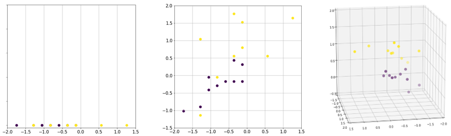
First, visualizing and analyzing a high-dimensional dataset to identify patterns and gain insights is difficult. For example, it is easier to visualize and analyze two-dimensional data than three-dimensional data. Beyond three dimensions, the analysis is more difficult and it is not possible to visualize the data. Second, some datasets may contain redundant features and features that are not relevant to solving the problem. These features should be removed because they do not add additional information to the prediction. Moreover, the features will incur unnecessary storage consumption and computation to the model training. Finally, the complexity of the problem and the machine learning models depends on the number of input dimensions as well as the number of instances. Although additional features may provide more information to the prediction, the volume of the feature space grows exponentially, thus the data becomes sparse. Figure 1 illustrates the issues of data sparsity. As we move from one dimension to three dimensions, there is more unoccupied space than the data points. As the number of dimensions grows, the data points appear to be equidistant and it becomes more difficult to cluster. Thus, given a high-dimensional dataset, the dataset should be analyzed to reduce it to a representation with lower dimensions.

Figure 1. Data density reduces exponentially as we move from one dimension to three dimensions. Data density refers to the amount of data points that can be stored per unit area.

Principal Component Analysis

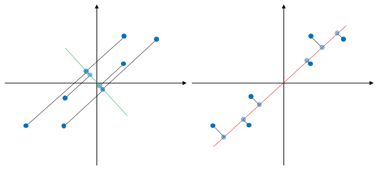
Principal component analysis (PCA) is one of the most commonly used dimensionality reduction method. In PCA, the data in the original $d$ -dimensional space is projected (or transformed) to $k$ -dimensional space, where $k < d$ . This is achieved by finding a hyperplane onto which to project the data. For simplicity, consider the data points in 2-d feature space as shown in Figure 2. The aim is to reduce the number of dimensions by projecting the data 1-d feature space. The figure shows two possible projections directions, one is onto a line in green color and the other one is onto a line in red color. The projected data points are indicated by blue circles. It can be seen that projecting data onto the green line results in overlapping data points while the red line results in data points that are scattered far away from each other. In other words, PCA seeks to find a direction in which to project the data that maximizes the variance of the data .

Figure 2. Projection direction on the left produces overlapping data points while projection direction on the right maximizes the variance of the data.

Let’s consider the best solution for projecting 2-d data to 1-d data. The vector that represents the best solution (line) that the data is to be projected onto is $\mathbf{w}_1$ . The vector is known as the first principal component. Thus, the projection of data $\mathbf{x}$ is defined by

$\mathbf{z} = \mathbf{w}_1^T\mathbf{x}$

We want the projected data to have a maximum variance. Thus, we seek to find $\mathbf{w}_1$ such that $\text{var}(\mathbf{w}_1^T\mathbf{x})$ is maximized subject to a constraint $\lVert \mathbf{w}_1 \rVert = 1$ , to ensure we obtain a unique solution. We rewrite the equation as follows:

$\text{var}(\mathbf{w}_1^T\mathbf{x})=\mathbf{w}_1^T\sum\mathbf{w}_1$

where $\sum$ is the covariance of $\mathbf{x}$ . We restate the optimization problem by applying Lagrange multipliers.

$\max \mathbf{w}_1^T \sum \mathbf{w}_1 - \lambda (\mathbf{w}_1^T\mathbf{w}_1 - 1)$

Taking the derivative with respect to $\mathbf{w}_1$ and setting it equal to zero.

$2\mathbf{w}_1 \sum - 2 \lambda \mathbf{w}_1 = 0$

Thus, $\sum\mathbf{w}_1 = \lambda \mathbf{w}_1$ . We can see that $\mathbf{w}_1$ is the eigenvector of $\sum$ and $\lambda$ is the corresponding eigenvalue. Because we want to maximize $\mathbf{w}_1 \sum \mathbf{w}_1$ , we choose the eigenvector with the largest eigenvalue for the maximum variance.

We can find the second vector $\mathbf{w}_2$ which is known as the second principal component. If the second component is solved, the 2-d dataset is not reduced, but transformed into a new 2-d representation. Note that the number of components that can be solved is equal to the number of dimensions of the data.

The second principal component should also maximize the variance, subject to $\lVert \mathbf{w}_2 \rVert = 1$ and $\mathbf{w}_2^T\mathbf{w}_1=0$ . We restate the problem by applying Lagrange multiplier. $\max \mathbf{w}_2^T \sum \mathbf{w}_2 - \lambda (\mathbf{w}_2^T\mathbf{w}_2 - 1) - \beta(\mathbf{w}_2^T\mathbf{w}_1 - 0)$

Taking the derivative with respect to $\mathbf{w}_2$ and setting it equal to zero.

$2\mathbf{w}_2 \sum - 2 \lambda \mathbf{w}_2 - \beta\mathbf{w}_1 = 0$

If we multiply the expression with $\mathbf{w}_1$

$2\mathbf{w}_2^T \sum \mathbf{w}_1 - 2 \lambda \mathbf{w}_2^T\mathbf{w}_1 - \beta\mathbf{w}_1^T\mathbf{w}_1 = 0$

We know that $\mathbf{w}_1^T\mathbf{w}_2 = 0$ and $\mathbf{w}_1^T \mathbf{w}_1 = 1$ . Then, the expression becomes $\beta \cdot 1 = 0$ . Thus, we know $\beta = 0$ .

We can reduce $2\mathbf{w}_2 \sum - 2 \lambda \mathbf{w}_2 - \beta\mathbf{w}_1 = 0$ to

$\sum \mathbf{w}_2 = \lambda \mathbf{w}_2$

where $\mathbf{w}_2$ is the eigenvector and $\lambda$ is the corresponding eigenvalue. Note that PCA is an unsupervised method in which it does not use the labels of the data. Thus, the resulting low dimesional representation may not be optimal for classification.

Solving for Eigenvectors and Eigenvalues

Suppose that

$\sum \mathbf{w} = \lambda \mathbf{w}$

where covariance matrix $\sum$ of data points $\mathbf{x}$ is defined by

$\sum = \frac{B^TB}{N-1}$

where $B=\mathbf{x} - JJ^T \mathbf{x}$ . $J$ is a $N\times1$ vector of ones.

Rewrite the above expression as follow:

$\mathbf{w}(\sum - \lambda I)=0$ where $I$ is an identity matrix

Solve $\text{det}(\sum - \lambda I)=0$ to obtain $\lambda$ .

Substitute $\lambda$ into $\mathbf{w}(\sum - \lambda I)=0$ to obtain $\mathbf{w}$ .

Numerical Example

Consider the following dataset

$\mathbf{x}=\begin{bmatrix}4 & 2\\5&5\\2&3\\8&7\\11&5\\10&8 \end{bmatrix}$

The mean of $\mathbf{x}$ is

$\mu=\begin{bmatrix}6.67&5\end{bmatrix}$

Mean normalize $\mathbf{x} - \mu$

$\tilde{\mathbf{x}} = \begin{bmatrix}-2.67 & -3\\-1.67&0\\-4.67&-2\\1.33&2\\4.33&0\\3.33&3 \end{bmatrix}$

Calculate $\sum=\frac{B^TB}{N-1}$ where $B=\tilde{\mathbf{x}}-JJ^T\tilde{\mathbf{x}}$ . Note that $B=$

$B=\begin{bmatrix}-2.67 & -3\\-1.67&0\\-4.67&-2\\1.33&2\\4.33&0\\3.33&3 \end{bmatrix} - \begin{bmatrix}1\\1\\1\\1\\1\\1\end{bmatrix}\begin{bmatrix}1\\1\\1\\1\\1\\1\end{bmatrix}^T \begin{bmatrix}-2.67 & -3\\-1.67&0\\-4.67&-2\\1.33&2\\4.33&0\\3.33&3 \end{bmatrix}=\begin{bmatrix}-2.67 & -3\\-1.67&0\\-4.67&-2\\1.33&2\\4.33&0\\3.33&3 \end{bmatrix}$

$\sum=\frac{B^TB}{6-1}=\begin{bmatrix}12.67&6\\6&5.2 \end{bmatrix}$

Find $\lambda$ by solving $\mathbf{w} (\sum - \lambda I)=0$ where $I=\begin{bmatrix}1&0\\0&1 \end{bmatrix}$

$\mathbf{w} (\begin{bmatrix}12.67&6\\6&5.2\end{bmatrix} - \lambda \begin{bmatrix}1&0\\0&1 \end{bmatrix})=0$

$\text{det}(\begin{bmatrix}12.67-\lambda&6\\6&5.2-\lambda\end{bmatrix})=0$

$(12.67-\lambda)(5.2-\lambda) - 6^2=0$

$\lambda^2 - 17.87\lambda + 29.88 = 0$

$\lambda_1 = 16.0$ and $\lambda_2=1.867$

$\lambda_1$ is the largest, hence the first principal component.

Substitute $\lambda_1 = 16.0$

$\begin{bmatrix}12.67&6\\6&5.2\end{bmatrix} \begin{bmatrix}w_1\\w_2 \end{bmatrix} = 16\begin{bmatrix}w_1\\w_2 \end{bmatrix}$

$12.67w_1 + 6w_2 = 16w_1$

$6w_1 + 5.2w_2 = 16w_2$

$w_1 = \frac{6}{3.33}w_2$

Let $w_2 = 1.0$ , thus $w_1 = \frac{6}{3.33} = 1.8$

$\mathbf{w} = \begin{bmatrix}1.8\\1 \end{bmatrix}$

The projected data $\mathbf{z}=\mathbf{w}^T \tilde{\mathbf{x}}$

Choosing $k$ Components

Total variance of the data is defined as

$\sigma^2_T = \sum_j^d \sigma^2_j$

where $\sigma^2_j = \frac{1}{N-1} \sum_{i=1}^N(z^i_j - \bar{z}_j)^2$ is the variance of component $j$ .

Explained variance is the ratio of variance of a principal component to the total variance, $\frac{\sigma^2_j}{\sigma^2_T}$ . We choose $k$ where the cumulative explained variance is 0.95 – 0.99.

References

[1] K. Pearson, “LIII. On lines and planes of closest fit to systems of points in space,” The London, Edinburgh, and Dublin Philosophical Magazine and Journal of Science, vol. 2, no. 11, pp. 559–572, Nov. 1901, doi: 10.1080/14786440109462720.

Introduction

Principal Component Analysis

Choosing Components

References

Choosing $k$ Components