Introduction
The artificial neural network architectures that have been discussed in the previous chapters are designed for 1-d and 2-d input data such as vectors and images. However, certain data types such as text and those generated by sensors contain sequential dependencies over time. A data point is dependent on data points that come before and after it. This can be seen in text data for any language, a sentence is constrained by the grammar of the language. The sequence of the words in a sentence exhibits a significant sequential correlation. For example, “I like playing football“, the word that comes after playing should be a sport, game or other similar nouns and it is very unlikely the following word is another verb. Thus, it is important that this sequential pattern or temporal structure is explored to improve the accuracy of the prediction. In the following section, we will discuss a specialized type of artificial neural network for processing a sequence of data. The neural network is called a recurrent neural network [1].
Recurrent Neural Networks
First, let us recall the artificial neural network. A neural network accepts an arbitrary number of inputs whereby each input is multiplied by a weight and the resultants are summed and passed to a non-linear activation function to produce an internal state of the neural network. The internal state is then fed to the subsequent layers to produce the predictive output. Now, consider a sequential dataset as shown below. The dataset has four input features, a target and the first column indicates the time the instances are collected which is every hour. Considering this is a sequential data, the target at a later time is mostly dependent on the inputs of the prior time.
 , hour , hour |  |  |  |  |  |
| 8.00 | 0.62 | 0.13 | 0.35 | 0.82 | 0 |
| 9.00 | 0.58 | 0.15 | 0.39 | 0.79 | 0 |
| … | … | … | … | … | … |
| 23.00 | 0.49 | 0.74 | 0.63 | 0.36 | 1 |
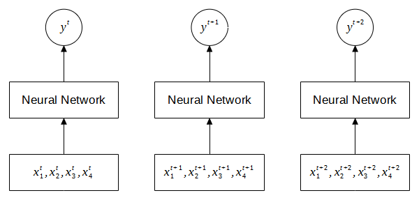
To predict the target is a straightforward task for an artificial neural network. We feed the input features to the neural network and the signals are propagated through the hidden layers to the output layer. Since, the data is time series, we can repeat the same steps for the subsequent time steps (rows) to predict the output. Figure 1 illustrates this approach whereby three input time steps are fed to the neural network. Note that the same neural network is used for each time step. At each time step, the input is given to the neural network and the predictive output is generated at that particular time step.
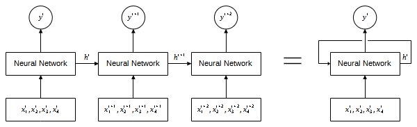
Although the neural network is able to learn the mapping between the features and the target, this approach assumes the data is non-sequential. This is because the neural network treats the instances as an individual isolated input, and consequently the relationship between the instances that is inherent in the sequence is not learned. To address this limitation, a neural network at time should be able to pass its computation (state) to the later time steps allowing the information to be used to generate the predictive outputs as shown in Figure 2. As we can see in the figure, each predictive output is a function of both the current input and the state from the previous time step. We can describe this model as a neural network with a recurrent connection as shown in the figure on the right.
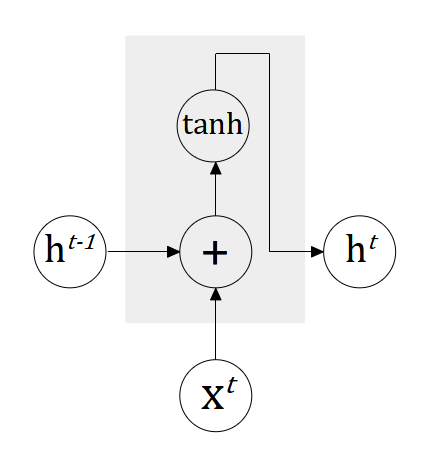
The recurrent neural network (RNN) is characterized by the recurrent connection (loop) which passes the information from one time step to another time step. The recurrent connection defines how the internal state of the neural network at each time step is updated. Specifically, the internal state is parameterized by a set of weights which will be learned as the sequences of data is processed over the course of training. Note that the weights are shared across the sequence which means the same weights are to be applied to each individual time step. Figure 3 illustrates the internal structure of a RNN.
Now, let’s look at the forward propagation of the RNN. Given a sequence of data  , the output for each time step
  to
to  is given as


where  is the hidden state of the RNN at time ,
  ,
,  and
and  are the weight matrices for input-to-hidden, hidden-to-hidden and hidden-to-output connections,
  and
and  are the biases and
  is typically tanh activation function.
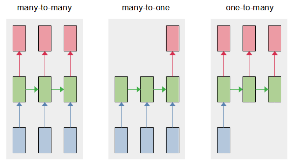
The above example is a RNN that maps an input sequence to an output sequence of the same length. This type of sequence modeling is known as many-to-many and a common application is machine translation. However, recurrent neural networks are flexible as the length of input and output can be configured to many-to-one and one-to-many as shown in Figure 4. Many-to-one takes a sequence of input and produces a single output. This type of sequence modeling is common in sentiment analysis where we want to determine the emotional tone of a document or a collection of sentences. One-to-many takes a single input and produces a sequence of output and a typical example of this modeling is image captioning. Given an input image, we want to generate a textual description of the image.
The training of recurrent neural networks is considerably more complex and difficult compared to standard neural networks. The total loss for many-to-one modeling is calculated based on the single output prediction. In the case of many-to-many and one-to-many, the total loss for a given input or sequence of input paired with the sequence of output is the sum of the losses over all the time steps. Computing the gradient of the loss function with respect to the weights is computationally expensive. The gradient computation begins with the forward propagation of the input sequence from left to right, followed by the backward propagation from right to left through the network. This learning algorithm is called backpropagation through time [2][3]. A major challenge in the training of recurrent neural networks is that the propagation of the gradients over many time steps may vanish [4].
Long Short-term Memory
Long short-term memory (LSTM) is a variant of RNN that was designed to overcome the problem of vanishing gradient when learning long-term dependencies [5]. LSTM is arguably the most widely used variant and it is applicable in various applications such as image captioning, machine translation, sentiment analysis and healthcare [6]. Similar to the standard recurrent neural network, LSTMs have the form of a chain repeating units. An LSTM unit consists of several gates that control the passing of information from one time step to another time step: forget gate, input gate and output gate. Figure 5 illustrates the flow of information and the interconnection of the gates. The key element in an LSTM unit is the cell  which remembers the information (state) at each time step. The cell is indicated by the horizontal line running through the top of the block. The cell state is updated by controlling the flow of information through the gates.
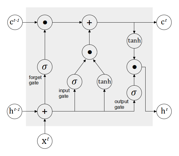
The forget gate accepts the input at time and the previous output time step  and determines which information needs to be filtered out from the previous cell’s state
  . This operation is performed by the sigmoid activation function, which outputs the value in the range of 0 (filter out) and 1 (keep).

where  and
and  are weight matrices that are learned.
The input gate is responsible for storing information in the current cell state based on the current input and the output of the previous time step . The operation involves activation functions, sigmoid and tanh. The sigmoid activation function decides which relevant information to be retrieved and the tanh activation function creates the candidate vector which will be used to update the cell state.


The cell state is updated via the following computation.

where  is element-wise multiplication.
The output gate accepts the current input and the output of the previous time step and combines them with the cell state . The computation of the output is given as follows.


Gated Recurrent Unit
Gated recurrent unit (GRU) is another popular variant of RNN. It is similar to LSTM whereby gating mechanism are used to control the flow of information from one time step to another time step. However, GRU has a relatively simpler architecture whereby it has two gates and does not store the state of each time step. Hence, the network has fewer parameters and is faster in terms of computation and training [7]. A GRU unit has two gates: reset gate and update gate. Figure 6 illustrates the interconnection of the gates.
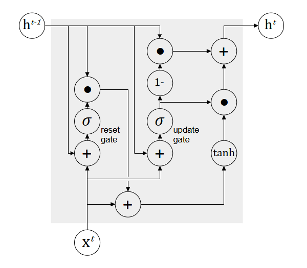
The reset gate takes the previous hidden state and decides which information to be ignored and processed with the current input to update the hidden state.

The update gate is computed similarly to the reset gate. However, it has a different usage whereby it controls how much information will be carried over from the previous hidden state to the current hidden state during the hidden state update.

Then, the hidden state at time is updated as follows.

where  is given by

Discussion
Gated recurrent neural networks such as LSTM and GRU are capable of learning long dependencies due to the additive component to update the hidden state from  to . Unlike RNN which replaces the hidden state with a new value computed from the current input and previous hidden state, LSTM and GRU update the current hidden state by adding the existing value with a new value. The additive component comes with several advantages. First, any important features that are extracted by the gating mechanism are not overwritten due to the addition operation. Thus, it is easy for each LSTM or GRU unit to store important features in the long sequence of inputs. Secondly, the additive component creates a direct connection between temporal units. This allows the error to be backpropagated easily to the earlier temporal units, without passing through the non-linear activation functions which may cause the vanishing gradient.
Despite their similarities, LSTM and GRU have a few differences. Both LSTM and GRU units control the amount of information flowing from the previous time step. However, the GRU unit does not independently control the new candidate activation while the LSTM unit directly controls the new candidate activation being added to the cell state. LSTM unit controls the amount of information to be passed to the next unit by the output gate. GRU unit fully exposes the hidden state to the next unit without any control.
References
[1] D. E. Rumelhart, G. E. Hinton, and R. J. Williams, “Learning representations by back-propagating errors,” Nature, vol. 323, no. 6088, Art. no. 6088, Oct. 1986, doi: 10.1038/323533a0.
[2] D. E. Rumelhart and J. L. McClelland, “Learning Internal Representations by Error Propagation,” in Parallel Distributed Processing: Explorations in the Microstructure of Cognition: Foundations, MIT Press, 1987, pp. 318–362. Accessed: Oct. 17, 2022. [Online]. Available: https://ieeexplore.ieee.org/document/6302929
[3] P. J. Werbos, “Generalization of backpropagation with application to a recurrent gas market model,” Neural Networks, vol. 1, no. 4, pp. 339–356, Jan. 1988, doi: 10.1016/0893-6080(88)90007-X.
[4] S. Hochreiter, Y. Bengio, P. Frasconi, J. Schmidhuber, and others, “Gradient flow in recurrent nets: the difficulty of learning long-term dependencies.” A field guide to dynamical recurrent neural networks. IEEE Press In, 2001.
[5] S. Hochreiter and J. Schmidhuber, “Long Short-Term Memory,” Neural Computation, vol. 9, no. 8, pp. 1735–1780, Nov. 1997, doi: 10.1162/neco.1997.9.8.1735.
[6] G. Van Houdt, C. Mosquera, and G. Nápoles, “A review on the long short-term memory model,” Artif Intell Rev, vol. 53, no. 8, pp. 5929–5955, Dec. 2020, doi: 10.1007/s10462-020-09838-1.
[7] K. Cho et al., “Learning Phrase Representations using RNN Encoder–Decoder for Statistical Machine Translation,” in Proceedings of the 2014 Conference on Empirical Methods in Natural Language Processing (EMNLP), Doha, Qatar, Oct. 2014, pp. 1724–1734. doi: 10.3115/v1/D14-1179.