Regularization for Neural Network

The main problem in machine learning is how to ensure the predictive models perform well not only on the training set but also on new data. Numerous methods have been introduced to improve the model generalization. These methods are collectively known as regularization. This section presents some of the regularization methods for neural networks.

Parameter Norm Penalty

Parameter norm penalty limits the capacity of the model by regularizing the weights of the neural network. The regularization is performed by adding a penalty term consisting of the weights to the loss function.

$J(\mathbf{w}) = \frac{1}{N} \sum_{i=1}^{N} L(y^i,\hat{y}^i) + \frac{\lambda}{2} \sum_l \lVert \mathbf{w}^{(l)} \rVert_2 ^2$

where $\lVert \mathbf{w} \rVert_2 ^2 = \sum_i \sum_j (w_{ij}^{(l)})^2$ , $\lambda$ is the shrinkage parameter and $L(y^i,\hat{y}^i)$ is the loss function whereby it could be the mean squared error or negative log-likelihood or other functions depending on the prediction problems.

The penalty term penalizes the weights of the neural network from going too large. This is because, when the training algorithm minimizes $J(\mathbf{w})$ , it will minimize both the loss function and the weights of the neural network. This may cause some of the weights to be close to zero especially if the shrinkage parameter is set to a large value. As a result, units with weight values close to zero switch off. This reduces the chance of overfitting because the neural network capacity is reduced.

The derivative of objective function $J(\mathbf{w})$ is

$\frac{\partial J(\mathbf{w})}{\partial w_{ij}^{(l)}}=\frac{\partial L(y^i,\hat{y}^i)}{\partial w_{ij}^{(l)}} + \lambda w_{ij}^{(l)}$

The weight update is

$\begin{aligned} w_{ij}^{(l)} &:= w_{ij}^{(l)} - \alpha (\frac{\partial L(y^i,\hat{y}^i)}{\partial w_{ij}^{(l)}} + \lambda w_{ij}^{(l)}) \\ &:= w_{ij}^{(l)} - \alpha \frac{\partial L(y^i,\hat{y}^i)}{\partial w_{ij}^{(l)}} - \alpha \lambda w_{ij}^{(l)} \\ &:= w_{ij}^{(l)} (1 - \alpha \lambda) - \frac{\partial L(y^i,\hat{y}^i)}{\partial w_{ij}^{(l)}} \end{aligned}$

As we can see above, the term $w_{ij}^{(l)} (1 - \alpha \lambda)$ has the effect where $w_{ij}^{(l)}$ is decreasing for every update because by the weight is update by the fraction of itself because $(1 - \alpha \lambda) < 0$ .

Early Stopping

When training a neural network, the training loss and validation loss decrease over time. However, after some time, the validation loss begins to increase indicating the model is overfitting the data. Early stopping is a method to terminate the training algorithm before the overfitting occurs. The model is overfitting the data is detected based on the evaluation of the validation set. For each iteration, after the backpropagation, the validation set is used to evaluate the model performance by calculating the validation loss or validation accuracy. The performance metric is used to determine if the model’s performance is improving or not. Every time the performance is improving, we store a copy of the model’s parameters. When the model performance is not improving and the training algorithm is terminated, we return the stored parameters. The early stopping algorithm is given as follows. $p$ is the number of epochs we will wait before the training is terminated if no improvement is observed. The parameter is known as “patience”.

Initialize 
Initialize 



for  to max_epoch do
   update  by performing backpropagation
    ValidationSetError
   if  then
      
      
      
   else
      
   if  then
      terminate loop

Dropout

One of the approaches to improve the accuracy of the prediction is to build several predictive neural networks and combine the predicted values via averaging. However, training a diverse set of neural networks is difficult and expensive due to the challenging task of finding the optimal hyperparameters. Furthermore, neural networks typically require a large number of training instances. Thus, training several neural networks may not be feasible because there may not be enough data to create different subsets to train the networks.

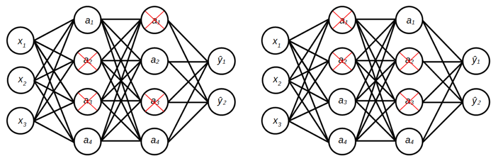
Dropout is a regularization method that approximately ensembles multiple neural networks with different architectures [1]. Dropout works by randomly eliminating a number of units in a hidden layer during the training of the neural network. The method defines a probability of a unit being dropped in a layer. For example, if the probability is set to 0.5, all the units in the layer are dropped at a 0.5 rate. For each weight update, after the instances are loaded into the mini-batch, a set of units of each layer is randomly sampled to be dropped. The mini-batch is then loaded to the reduced neural network for forward and backpropagation. This can be seen as estimating the weights of different network architectures since different sets of units are eliminated as shown in Figure 1. Thus, the randomly dropping out units has the effect of training and evaluating exponentially many different neural networks. At test time, the resulting neural network is used without dropout.

Another advantage of dropout is preventing the co-adaptation of units in the neural network [2]. Co-adaptation occurs when some units are highly dependent on other units which means when the independent units fail to produce the correct activations, the dependent units are affected as well, hence the neural network will fail to correctly predict the inputs. With dropout, no units can be too “powerful” due to the random elimination, thus forcing all units in the neural network to take part in the prediction.

Figure 1. Different units are randomly dropped for each backpropagation.

Let $p$ the probability of units to be retained. Therefore, the drop rate is $1-p$ . $\mathbf{r}$ is the vector of Bernoulli whereby each element in the vector has the probability of $p$ of being 1. Note that Bernoulli variable can take either 0 (failure) or 1 (success) with the probability of being success is $p$ .

$\mathbf{r}=\text{Bernoulli}(p)$

During training, the forward propagation with dropout is implemented as follows:

$\tilde{\mathbf{a}}^{(l)} = \frac{\mathbf{r}^{(l)} * \mathbf{a}^{(l)}}{p}$

$\mathbf{z}_i^{(l+1)} = \mathbf{w}_i^{(l)} \tilde{\mathbf{a}}^{(l)} + w_{i0}^{(l)}$

$\mathbf{a}_i^{(l+1)} = g(\mathbf{z}_i^{(l+1)})$

where $*$ is the element-wise multiplication, $\mathbf{a}^{(l)}$ is the activation of the hidden layer $l$ and $\tilde{\mathbf{a}}^{(l)}$ is the reduced activation of the hidden layer. The activation of the layer is multiplied element-wise with the vector of Bernoulli. This causes some of the activations to be zero. The reduced activation is scaled with $\frac{1}{p}$ to ensure the expectation of the input to the next layer remains the same. The reduced activation is then used as input to the next layer. At test time, the forward propagation is implemented without dropout.

Batch Normalization

We commonly used mini-batch gradient descent to train neural networks. In mini-batch gradient descent, the weight update is performed for every mini-batch and each batch may contain data from different distributions. Furthermore, the distribution of the inputs to each hidden layer may change after each mini-batch when the weights are updated. This could slow down the training process because each layer needs to adapt to the new distribution.

Batch normalization is a regularization method that incorporates normalization into the model architecture [3]. Specifically, the method allows each layer to perform normalization on the layer’s output for each mini-batch. The layer normalization has the effect of stabilizing and speed up the training process.

Let $z_i$ denotes the summation of the weighted inputs of unit $i$ of a hidden layer. We calculate the mean of $z_i$ over the mini-batch.

$\bar{z}_i = \sum_{m=1}^{M} z_i^m$

where $M$ is the number of instances in the mini-batch. The variance of the mini-batch is

$\sigma_i^2 = \frac{1}{M} \sum_{m=1}^M (z_i^m - \bar{z}_i)$

The normalization is given as follows:

$\acute{z}_i^m = \frac{z_i^m - \bar{z}_i}{\sqrt{\sigma_i^2 + \epsilon}}$

where $\epsilon$ is a small constant for computation stability. To allow flexibility to the layer to adjust the distribution of the activations, a pair of trainable parameters $\gamma$ and $\beta$ are introduced as follows:

$\tilde{z}_i^m = \gamma_i \acute{z}_i^m + \beta_i$

The parameters are estimated during training. Batch normalization can be applied before or after the non-linearity (activation function). Note that the authors applied the normalization before non-linearity.

References

[1] N. Srivastava, G. Hinton, A. Krizhevsky, I. Sutskever, and R. Salakhutdinov, “Dropout: A Simple Way to Prevent Neural Networks from Overfitting,” Journal of Machine Learning Research, vol. 15, no. 56, pp. 1929–1958, 2014.

[2] G. E. Hinton, N. Srivastava, A. Krizhevsky, I. Sutskever, and R. R. Salakhutdinov, “Improving neural networks by preventing co-adaptation of feature detectors,” arXiv preprint arXiv:1207.0580, 2012.

[3] S. Ioffe and C. Szegedy, “Batch normalization: accelerating deep network training by reducing internal covariate shift,” in Proceedings of the 32nd International Conference on International Conference on Machine Learning – Volume 37, Lille, France, Jul. 2015, pp. 448–456.