Supervised Learning – Halim Noor

Introduction

Supervised learning is the most commonly used approach to machine learning. Some of the popular supervised learning applications are e-mail spam detection, optical character recognition and face recognition. In supervised learning setting, we are given a labeled dataset or in other words, the dataset comes in pairs of $(\mathbf{x}^i,y^i)$ , where $i=1,2,...,N$ and $N$ is the number of samples or instances in the dataset. Each input $\mathbf{x}^i$ is a $d$ -dimensional vector, $\mathbf{x}^i=(x_1,x_2,…,x_d)$ where each element, ${x_j}$ is a feature describing the $i$ -th input.

Feature Vector

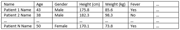
Let us consider a dataset consisting of $N$ patient data as shown in Figure 1. The dataset is arranged in the form of a table whereby the columns are the features of the patients. A row represents a patient. This is known as a structured data. The feature vector of $i$ th patient, $\mathbf{x}^i=(x_1, x_2,...,x_d)$ where feature ${x_1}^i$ refers to $i$ th patient’s name, ${x_2}^i$ refers to $i$ th patient’s age, ${x_3}^i$ refers to $i$ th patient’s gender, ${x_4}^i$ refers to $i$ th patient’s height, etc. The features can be categorical or numerical.

A dataset of $N$ text documents such as e-mails, review etc. Text data is typically converted into a form which can be used as input to the machine learning models. One of the commonly used methods to represent text data is the bag-of-words. The bag-of-words converts the text data into a sequence of integers based on the occurrence of the words in the document as shown in Figure 2. A bag-of-words feature vector, $\mathbf{x}^i=(x_1, x_2,...,x_d)$ where $d$ is the number of words in the whole corpus, ${x_1}^i$ refers to the number of occurrence of word 1 in $i$ th document, ${x_2}^i$ refers the number of occurrence of word 2 in $i$ th document, etc.

Figure 2. Text data with its bag-of-words representation.

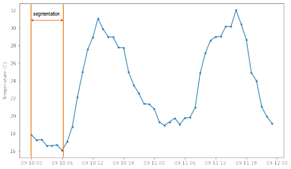
Time series data is a sequence of data that is ordered by time. For example, temperature sensors that are used to monitor the temperature of the environment generate measurements every 30 minutes. The sequence of the values over time is important because it contains information such as the trend and seasonality. A single sample (measurement) does not carry sufficient information to perform predictions. Therefore, for time series data, usually, we segment or group several samples, enough to contain the temporal information, and the segmentation is used for the prediction as shown in Figure 3. The subsequent segmentation may partially overlap the previous segmentation. The feature vector is a segmentation, $\mathbf{x}^i=(x_1, x_2,...,x_d)$ where $d$ is the size of segmentation, $x_j^i$ refers to $j$ th sample in the $i$ th segmentation.

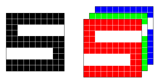
Figure 3. A segment of time series data is considered as an input for predictions.

Finally, prediction with machine learning may involve image data. Image data is a collection of pixels arranged in rows and columns. The arrangement of the pixels defines the visual information or known as spatial structure. The image size determines the number of pixels. The image can be a grayscale image or a color image. For grayscale images, each pixel has one value representing the intensity of the pixel. The range of value is $[0,255]$ whereby 0 represents black and 255 represents white. For color images, each pixel has three values for red, green and blue. The combination of the values defines the color of the pixel. The feature vector $\mathbf{x}^i=(x_{1,1}, x_{1,2},.x_{1,3}..,x_{d,1},x_{d,2},x_{d,3})$ where $x_{j,1}$ , $x_{j,2}$ and $x_{j,3}$ refer to red, green and blue of $j$ th pixel and $d$ is the number of pixels in the image.

Figure 4. Each pixel value in a grayscale image is the intensity while each pixel value in a color image has three values for red, green and blue.

Types of Supervised Learning

The output or response variable $y^i$ can be either a categorical or a numerical variable. If the output is a categorical variable, $y^i$ is a finite set, $y\in\{{1,2,...,C}\}$ where $C$ denotes the number of labels (classes) such as low, medium and high. This problem is known as multiclass classification. In the case of $C=2$ , say yes and no, the problem is known as binary classification. If the output is a numerical value, $y\in\mathbb{R}$ such as house price and salary, the problem is known as regression. The following table summarizes the types of supervised learning problems

y^i\in\{{0,1}\} — Table 1. The supervised learning problems depend on the type of target or response variable.

y^i\in\{{-1,1}\} — Table 1. The supervised learning problems depend on the type of target or response variable.

The data points are generated by an unknown function $y=f(\mathbf{x})$ . The aim of supervised learning is to approximate (learn) the unknown function $\hat{f}$ given the dataset. With the approximated function, the output of a new data point $\mathbf{x}$ can be predicted $\hat{y}=\hat{f}(\mathbf{x})$ . The approximated function is also called hypothesis or predictive model. Note that the two terms will be used interchangeably. To learn a function, we choose an algorithm such as decision tree, support vector machine or k-nearest neighbors – there are more algorithms. By choosing an algorithm, we are making an assumption about the data that we are trying to learn.

Overfitting and Underfitting

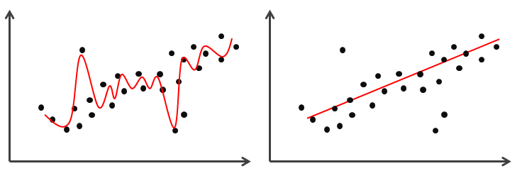
There are two problems that can be encountered when learning the hypothesis. The first problem is overfitting, whereby the hypothesis learns every minor variation in the data including the noise. This could easily happen when a highly flexible algorithm is used such as decision tree, support vector machine and neural network. Overfitting causes the hypothesis to become too specific, consequently failing to predict new data. Conversely, we do not want a hypothesis that failed to capture the variation in the data, which is known as underfitting. This could happen when a simple algorithm is used such as linear regression, logistic regression and linear discriminant analysis. The two problems are illustrated in Figure 5.

Figure 5. (left) Overfitting is when every minor variation in the data is learned. (right) Underfitting is when the pattern of the data is not learned.

Loss Function

When approximating or learning the hypothesis $\hat{f}(\mathbf{x})$ , we want a hypothesis that makes the least mistakes, which means the one with minimum incorrect classification or the best estimation. In machine learning, the mistakes or errors can be quantified using several loss functions. A loss function tells how bad a hypothesis is in performing the prediction.

Zero-one loss

The simplest loss function, which typically used to quantify incorrect classification. The loss function calculates the summation of every misclassification and normalizes the summation by the number of instances. The zero-one loss is defined as follows:

$J_{0-1}(\hat{f})=\frac{1}{N} \sum_{i=1}^{N} I(y^i\neq \hat{f}(\mathbf{x})^i)$ where $I(c)=\begin{cases} 1 & \text{if } c \text{ is True} \\ 0 & \text{if } c \text{ is False} \end{cases}$

Negative Log-Likelihood

Another loss function for classification problems is the negative log-likelihood or also known as cross-entropy. The loss function measures the difference between the probability distribution of the response and the prediction. For binary classification, the loss function is defined as follows:

$J_{nll}(\hat{f})= -\frac{1}{N} \sum_{i=1}^{N} [y^i \log_e{\hat{f}(\mathbf{x}^i)} + (1-y^i) \log_e{(1-\hat{f}(\mathbf{x}^i))}]$

For multiclass classification, the loss function is defined as follows:

$J_{nll}(\hat{f}) = -\frac{1}{N} \sum_{i=1}^N \sum_{c=1}^C y_c^i \log_e{\hat{f}_c(\mathbf{x}^i)}$

Squared loss

The squared loss function is typically used to calculate the errors in regression problems. The loss function calculates the squared difference between the response and the predicted value and normalizes it by the number of instances. The squaring amplifies large prediction errors, thus encouraging the hypothesis not to make many mistakes. Conversely, if the prediction is close to being correct, the error will be very small, and little attention will be given to further improving the prediction.

$J_{sq}(\hat{f})=\frac{1}{N} \sum_{i=1}^{N} (y^i-\hat{f}(\mathbf{x})^i)^2$

Often, we build a set of hypotheses using different algorithms. This is crucial because there is no single algorithm that will always give the best performance for every problem. This is the No Free Lunch Theorem. Given the loss function, we choose a hypothesis, $\hat{f}$ from a set of hypotheses $H$ that minimizes the loss function.

$\hat{f}=\arg \min_{h\in{H}} J(\hat{f})$

Performance Metrics

Besides the error, specifically in classification problems, we can evaluate the performance of the hypothesis by analyzing the number of correct and incorrect classifications in a specific table form called confusion matrix. Figure 6 shows a confusion matrix for a binary classification problem, where the two classes are “Yes” and “No”. The number of correctly classified of “Yes” class is represented by True Positive while the number of correctly classified of “No” class is represented by True Negative. The number of incorrect classifications are represented by False Negative and False Positive. False Negative is the number of instances belonging to “Yes” which are misclassified as “No”. False Positive is the number of instances belonging to “No” which are misclassified as “Yes”.

	Yes	No
Yes	True Positive (TP)	False Negative (FN)
No	False Positive (FP)	True Negative (TN)

Figure 6. Confusion matrix

Several performance metrics can be derived from the confusion matrix. Here we look at the four commonly used metrics. The first metric is called Recall. Recall is the fraction of relevant instances that are correctly classified. Recall is defined as follows:

$\text{Recall}=\frac{TP}{TP+FN}$

The second commonly used metric is Precision. Precision is the fraction of relevant instances among the classified instances. Precision is defined as follows:

$\text{Precision}=\frac{TP}{TP+FP}$

The F-score measure is derived from Recall and Precision as follows:

$\text{F-score}=2 \cdot \frac{\text{Recall} \cdot \text{Precision}}{\text{Recall} + \text{Precision}}$

Lastly, the accuracy of the hypothesis is defined as follows:

$\text{Accuracy}=\frac{TP+TN}{TP+TN+FP+FN}$

For regression problems, the squared loss is typically used to evaluate the hypothesis. In addition to squared loss, absolute error is also used in model evaluation. The metrics are defined as follows:

$\text{MSE}=\frac{1}{N} \sum_{i=1}^N (y^i - \hat{f}(\mathbf{x}^i))^2$

$\text{MAE} = \frac{1}{N} \sum_{i=1}^N \lvert y^i - \hat{f}(\mathbf{x}^i) \rvert$

The absolute difference between response and the predicted value is taken to avoid the canceling of positive and negative magnitude. The metric tells us how far the hypothesis prediction deviates from the response. Another commonly used performance metric is the $\text{R}^2$ ( $\text{R}$ -squared). $\text{R}^2$ measures the goodness of fit of the hypothesis. It measures the ratio of the hypothesis error to the worse or baseline error which is the average of the response. $\text{R}^2$ can be written as follows:

$\text{R}^2=1-\frac{\text{SS}_{res}}{\text{SS}_{tot}}$

where $\text{SS}_{res}$ is the sum of squared error of the hypothesis and $\text{SS}_{tot}$ is the sum of squared error of the baseline. The errors are defined as follows:

$\text{SS}_{res} = \sum_{i=1}^N (y^i - \hat{f}(\mathbf{x}^i))^2$

$\text{SS}_{tot} = \sum_{i=1}^N (y^i - \bar{y})^2$

where $\bar{y}=\frac{1}{N} \sum_{i=1}^N y^i$

$\text{R}^2$ provides a measure in the range of 0 and 1. $\text{R}^2=1$ indicates a perfect hypothesis while $\text{R}^2=0$ indicates a worst possible hypothesis.

Training, Validation and Test Sets

We not only want the hypothesis to perform well on the data that it has been trained to predict. Most importantly, the hypothesis must perform well on new data. The ability of the hypothesis to perform well on data that it has not seen before is known as generalization. To achieve generalization, the dataset is split into three subsets, namely training set, validation set and test set. This method is called hold-out method.

Hold-out Method

A portion of the data is hold-out for validation and evaluation. The training set will have a larger portion of the instances, typically around 60% – 80% of the dataset. The remaining instances are split into validation and test sets as shown in Figure 7. The dataset can also be split first into training and test sets. Then, the training set is further split into training and validation sets. The split ratio varies from one application or problem to another. The commonly used split ratio are 6:2:2, 7:1:2, 8:1:1.

Figure 7. The dataset is split into training, validation and test sets.

The training set is used to learn the hypothesis. The machine learning algorithms have several parameters that need to be set and fine-tuned to obtain an optimal hypothesis. To find the optimal parameters, the validation set is used to validate the hypothesis. If the loss is too large, the hypothesis will be retrained with different parameters using the training set, and the newly trained hypothesis is validated using the validation set. Once, an optimal hypothesis is obtained, the test set is used to evaluate the performance of the hypothesis. The test loss is the generalization errors.

$K$ -fold Cross Validation

Ideally, if we have sufficient data, a portion of instances can be set aside for validation. But data is often scarce and we don’t have sufficient training and validation instances to make a reliable estimate of the error. A popular method to solve this problem is cross-validation where the dataset is split into training and test sets. Then, the cross-validation is employed to train the hypothesis using the training set. We split the data into $K$ partitions of equal-sized, say $K=5$ as shown in Figure 8.

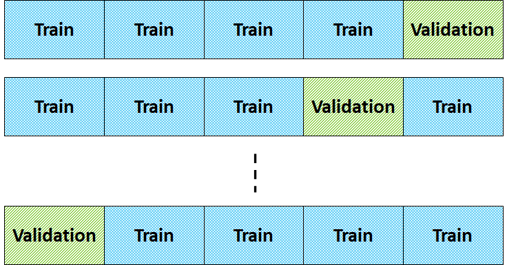
The hypothesis is learned using $K-1$ partitions and the $k$ th partition is used as the validation set. We repeat this for $k=1,2,...,K$ and the error estimate is the average error over $K$ repetition. The common value of $K$ is 3, 5 and 10. When $K=N$ , this is known as leave-one-out cross-validation whereby all instances except the $k$ th instance are used to learn the hypothesis.

Summary

In summary, the dataset is split into training set, $D_{tr}$ , validation set, $D_{vd}$ and test set, $D_{te}$ .

A set of hypotheses, $H$ are trained using the $D_{tr}$ .

$\text{Learning}: \hat{f}=\arg\min_{\hat{f} \in{H}} \frac{1}{\lvert D_{tr}\rvert} \sum_{i=1}^{\lvert D_{tr}\rvert} l(y^i,\hat{f}(\mathbf{x^i}))$

where $l$ can be zero-one loss or squared loss.

Choose a hypothesis that minimizes the validation loss.

$\text{Validating}: \hat{f}=\arg\min_{\hat{f} \in{H}} \frac{1}{\lvert D_{vd}\rvert} \sum_{i=1}^{\lvert D_{vd}\rvert} l(y^i,\hat{f}(\mathbf{x^i}))$

where $l$ can be zero-one loss or squared loss.

Evaluate the chosen hypothesis, $\hat{f}^*$ on the test set and calculate the generalization error, $\epsilon$ .

$\text{Test}: \epsilon=\frac{1}{\lvert D_{te}\rvert} \sum_{i=1}^{\lvert D_{te}\rvert} l(y^i,\hat{f}(\mathbf{x^i}))$

where $l$ can be zero-one loss or squared loss.

Binary classification	$y^i\in\{{0,1}\}$ or $y^i\in\{{-1,1}\}$	E.g. brain cancer detection (yes or no)
Multiclass classification	$y^i\in\{{1,2,...,C}\}$ where $C$ is the number of classes and $C>2$	E.g. classifying vehicles (lorry, van, car and motorcycle)
Regression	$y^i\in\mathbb{R}$	E.g. predicting house price, salary