Support Vector Machine

Introduction

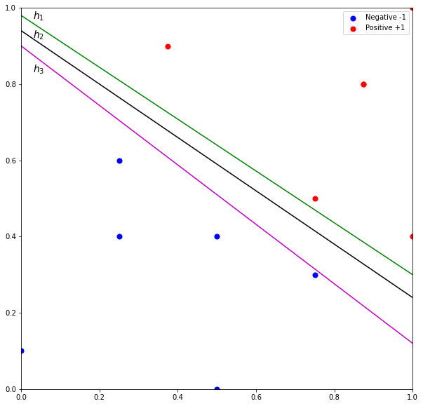
Perceptron seeks to find a hyperplane that can linearly separate the data points into their classes. But perceptron does not guarantee the hyperplane is the optimal solution. Figure 1 illustrates three possible solutions among an almost infinite number of possible hyperplanes. Although the hyperplanes perfectly separate the data points, misclassification could easily occur. For example, it is very likely for test points belonging to NEGATIVE class to be above hyperplane $h_3$ . Similarly, test points belonging to POSITIVE class could appear below hyperplane $h_1$ . As for $h_2$ , although the hyperplane appears to be a “better” hyperplane, the decision boundary is closer to POSITIVE class. Thus, the misclassification rate would increase especially for POSITIVE class.

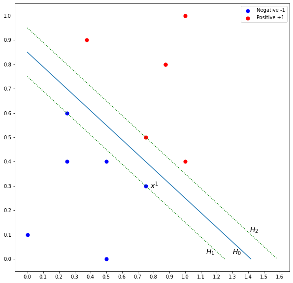
Figure 1. Three possible hyperplanes can linearly separate the data points perfectly.

Support vector machine (SVM) finds an optimal hyperplane that best separates the data points. This optimal solution is the hyperplane that is far away from the data points of both classes. To this end, SVM introduces the notion of margin which is illustrated in Figure 2. The margin is defined by the distance from the parallel dotted lines that are crossing the closest data points of both classes. The hyperplane is in the middle indicated by the blue line. The optimal hyperplane is the one that maximizes the margin of the training instances. The idea is if the margin is maximized, the hyperplane will be far away from the data points of both sides and reduce the chance of misclassification.

Figure 2. An optimal hyperplane that separates the two classes.

How do we find the margin? Given hyperplane $H_0$ that separates the two classes, we know that $H_0$ is equidistant from hyperplane $H_1$ and $H_2$ . $H_0$ is defined by

$\mathbf{w}^T\mathbf{x} + b=0$

where $\mathbf{x}$ is the feature vector and $\mathbf{w}$ and $b$ are the parameters of the hyperplane. For each instance $x^i$ , we know that

$\mathbf{w}^T\mathbf{x}^i + b \geq +1$ for all $\mathbf{x}^i$ belong to class $+1$

$\mathbf{w}^T\mathbf{x}^i + b \leq -1$ for all $\mathbf{x}^i$ belong to class $-1$

These are the constraints that need to be respected in order to select the optimal hyperplane. The first constraint states that all instances belonging to class $+1$ must be above $H_2$ and the second constraint states that all instances belonging to class $-1$ must be below $H_1$ . By not violating these constraints, we are selecting two hyperplanes (that define the margin) with no data points in between them. Let’s simplify the constraints. We multiply the first constraint on both sides with $y^i$ .

$y^i(\mathbf{w}^T\mathbf{x}^i + b) \geq y^i(+1)$

We know that for all $x^i$ belonging to class $+1$ , $y^i$ is $+1$ . Thus, the constraint becomes

$y^i(\mathbf{w}^T\mathbf{x}^i + b) \geq +1$

We do the same for the second constraint.

$y^i(\mathbf{w}^T\mathbf{x}^i + b) \leq y^i(-1)$

We know that for all $x^i$ belonging to class $-1$ , $y^i$ is $-1$ . Thus, the constraint becomes

$y^i(\mathbf{w}^T\mathbf{x}^i + b) \geq +1$

Therefore, we can combine the two constraints as follows

$y^i(\mathbf{w}^T\mathbf{x}^i + b) \geq +1$ for all instances $\mathbf{x}^i$ .

Figure 3. The margin is maximized to obtain the optimal hyperplane.

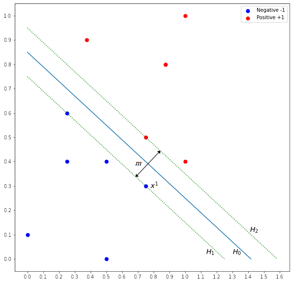
$m$ is the margin as shown in Figure 3. We know that $\mathbf{w}$ is a vector that is perpendicular to the hyperplanes. If the unit vector of $\mathbf{w}$ is multiplied with $m$ , we get a vector $\mathbf{v}$ , where it has the same direction as $\mathbf{w}$ and with a distance equal to $m$ . Let the unit vector be $\mathbf{u}=\frac{\mathbf{w}}{\lVert w \rVert}$ , thus $\mathbf{v}=m \mathbf{u}$ .

We know that $H_1$ and $H_2$ are

$H_1: \mathbf{w}^T\mathbf{x} + b = -1$

$H_2: \mathbf{w}^T\mathbf{x} + b = +1$

Let $\mathbf{x}^1$ is a data point on $H_1$ . If we add $\mathbf{x}^1$ with $\mathbf{v}$ , the resultant is a point on $H_2$ .

$\mathbf{x}^2 = \mathbf{x}^1 + \mathbf{v}$

We can write $H_2$ as follows:

$\mathbf{w}^T(\mathbf{x}^1 + \mathbf{v}) + b = 1$

$\mathbf{w}^T(\mathbf{x}^1 + m \frac{\mathbf{w}}{\lVert w \rVert}) + b = 1$

$\mathbf{w}^T\mathbf{x}^1 + b + m \frac{\lVert w \rVert^2}{\lVert w \rVert}= 1$

$\mathbf{w}^T\mathbf{x}^1 + b + m \lVert w \rVert = 1$

We know that $\mathbf{w}^T\mathbf{x}^1 + b = -1$ . We can rewrite the equation and solve for $m$ .

$m \lVert w \rVert= 2$

$m = \frac{2}{\lVert w \rVert}$

Therefore, margin $m$ is maximized when $\lVert w \rVert$ is minimized. For mathematical convenience, we change from minimizing $\lVert w \rVert$ to minimizing $\frac{1}{2} \lVert w \rVert^2$ .

$\min \frac{1}{2} \lVert w \rVert^2$ subject to $y^i(\mathbf{w}^T\mathbf{x}^i + b) \geq 1$ for $i=1,2,...,N$

You may skip the derivation of the solution and go to parameter solving.

We can solve the constrained optimization problem using quadratic programming [1]. Before that, we restate the optimization problem by applying Lagrange multiplier. Lagrange multiplier states that to find the maximum or minimum of a function $f(x)$ subjected to an equality constraint $g(x)$ , form the following expression $L$ , set the gradient of $L$ to zero and find the Lagrange multiplier (parameter) $\lambda$ .

$L(x) = f(x) - \lambda g(x)$

Substitute $f(x)$ and $g(x)$ .

$L_p = \frac{1}{2} \lVert w \rVert^2 - \lambda^i (y^i(\mathbf{w}^T\mathbf{x}^i + b) - 1)$ for all $i$ .

$L_p = \frac{1}{2} \lVert w \rVert^2 - \sum_{i=1}^{N} \lambda^i y^i(\mathbf{w}^T\mathbf{x}^i + b) + \sum_{i=1}^N \lambda^i$ .

Differentiate $L_p$ with respect to $w$ and $b$ , and set it to zero

$\frac{\partial L_p}{\partial w}=0$ , $w=\sum_{i=1}^{N} \lambda^i y^i \mathbf{x}^i$

$\frac{\partial L_p}{\partial b}=0$ , $\sum_{i=1}^{N} \lambda^i y^i = 0$

Substitute $w$ and $\sum_{i=1}^{N} \lambda^i y^i = 0$ into $L_p$ and simplify it.

$L_d = \frac{1}{2} (\sum_{i=1}^{N} \lambda^i y^i \mathbf{x}^i)^2 - \sum_{i=1}^{N} \sum_{j=1}^{N} \lambda^i \lambda^j y^i y^j (\mathbf{x}^i)^T \mathbf{x}^j + \sum_{i=1}^{N} \lambda^i$

$L_d = \sum_{i=1}^{N} \lambda^i - \frac{1}{2} \sum_{i=1}^{N} \sum_{j=1}^{N} \lambda^i \lambda^j y^i y^j (\mathbf{x}^i)^T \mathbf{x}^j$

Thus, the optimization problem becomes as follows.

$\max_{\lambda} [\sum_{i=1}^{N} \lambda^i - \frac{1}{2} \sum_{i=1}^{N} \sum_{j=1}^{N} \lambda^i \lambda^j y^i y^j (\mathbf{x}^i)^T \mathbf{x}^j]$

subject to $\lambda^i \geq 0$ and $\sum_{i=1}^{N} \lambda^i y^i = 0$ .

As we can see above, the objective function now depends only on the Lagrange multipliers which is easier to be solved. Upon solving the optimization problem, most Lagrange multipliers ( $\lambda^i=0$ ) will be zero, and only a few of them are non-zero. The data points with $\lambda>0$ are called the support vectors [2]. These support vectors lie on the edge of the margin which define the margin and the optimal hyperplane.

From the above, we see the solution for $\mathbf{w}$ has the form

$\mathbf{w}=\sum_{i=1}^{N} \lambda^i y^i \mathbf{x}^i$

We can use any data point on the edge of the margin to solve $b$ . However, typically we use an average of all the solutions for numerical stability.

$b = \frac{1}{\lvert S \rvert} \sum_{s \in S} y^s - \mathbf{w}^T \mathbf{x}^s$

where $S$ is the set of support vector indices. Given a test point $\mathbf{\acute{x}}$ , the predicted value is

$\hat{f}(\mathbf{x}) = \text{sign} (\mathbf{w}^T\mathbf{\acute{x}} + b)$

Soft Margin

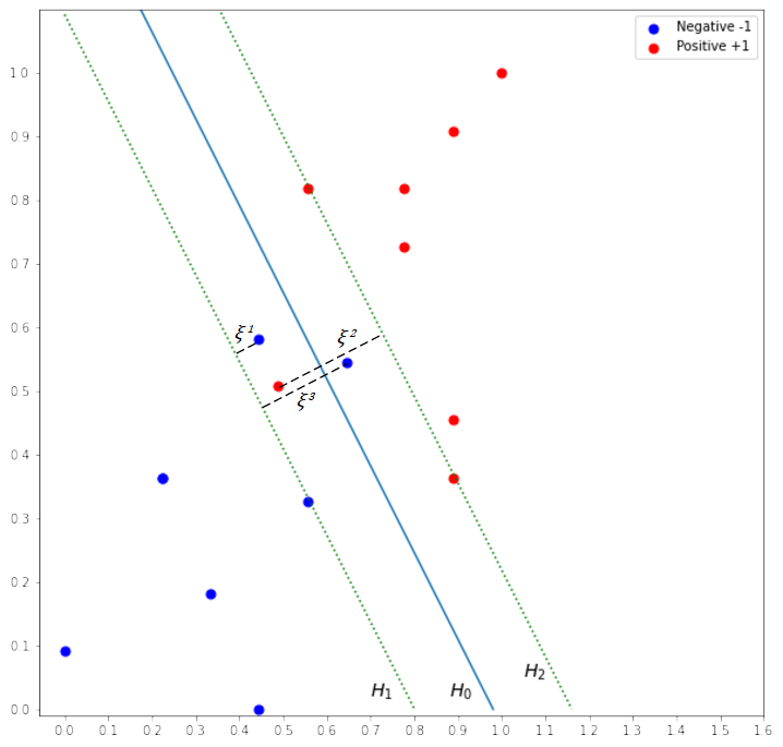
Real-world data are typically noisy and not linearly separable. When the data are not separable, the algorithm above will not be able to produce the solution to the problem. To handle non-separable data, we relax the constraints by allowing data points within the margin. Consider the margin in Figure 4. Three data points are allowed to be within the margin. These “errors” need to be quantified as indicated by $\xi^i$ and included in the constraints. The variable $\xi^i$ is known as slack variable. $\xi^i$ represents the amount of which the data points on the wrong side of the margin. If $\xi^i=0$ , the data point is on the right side. If $0 \leq \xi \leq 1$ , the data point is in the margin. If $\xi > 1$ , the data point is on the wrong side of the hyperplane.

Figure 4. Data points in the margin are errors that are included in the constraints.

The combined constraint is now defined as follows:

$y^i (\mathbf{w}^T\mathbf{x}^i + b) \geq 1 - \xi^i$ where $\xi^i \geq 0$ and $i=1,2,...,N$

The equation (constraint) implies that we define an error if the prediction is on the wrong side of margin boundary. This is called the hinge loss. Given the prediction $\hat{y}=(\mathbf{w}^T\mathbf{x}+b)$ , the loss function is defined as

$J_{hinge}(y,\hat{y})=\max(0,1-y\hat{y})$

By introducing the slack variables in the optimization problem, it is still possible to satisfy the constraint, albeit with some data points within or on the wrong side of the hyperplane. We add a term to the objective function which represents the total amount of which the data points on the wrong side of their margin.

$\min \frac{1}{2} \lVert w \rVert^2 + C \sum_{i=1}^N \xi^i$

subject to $y^i(\mathbf{w}^T\mathbf{x}^i + b) - 1 + \xi \geq 0$ and $\xi^i \geq 0$ for $i=1,2,...,N$

where $C$ is the regularization parameter to control the trade-off between maximizing the margin and minimizing the error. Small $C$ gives less importance to the error term, hence more mistakes are allowed, resulting in large margin. Conversely, large $C$ allows less mistakes resulting in small margin. You may skip the derivation of the solution and go to parameter solving.

Using Lagrange multiplier to formulate the optimization problem with respect to the Lagrange parameters.

$L_p = \frac{1}{2} \lVert w \rVert^2 + C \sum_{i=1}^N \xi^i - \sum_{i=1}^{N} \lambda^i (y^i(\mathbf{w}^T\mathbf{x}^i + b) - 1 + \xi^i) - \sum_{i=1}^N \mu^i \xi^i$

where $\mu^i$ is the Lagrange multiplier for constraint $\xi^i \geq 0$ .

Differentiate $L_p$ with respect to $w$ , $b$ and $\xi$ , and set it to zero.

$\frac{\partial L_p}{\partial w}=0$ , $w=\sum_{i=1}^{N} \lambda^i y^i \mathbf{x}^i$

$\frac{\partial L_p}{\partial b}=0$ , $\sum_{i=1}^{N} \lambda^i y^i = 0$

$\frac{\partial L_p}{\partial \xi}=0$ , $C - \lambda^i - \mu^i = 0$

Since $\mu^i \geq 0$ , this implies $0 \leq \lambda^i \leq C$ .

Substitute the derivatives into $L_p$ and simplify it.

$L_d = \sum_{i=1}^{N} \lambda^i - \frac{1}{2} \sum_{i=1}^{N} \sum_{j=1}^{N} \lambda^i \lambda^j y^i y^j (\mathbf{x}^i)^T \mathbf{x}^j$

subject to $\sum_{i=1}^{N} \lambda^i y^i = 0$ and $0 \leq \lambda \leq C$ .

Upon solving the optimization problem using quadratic programming, data points that lie on the correct side of the hyperplane, their corresponding $\lambda^i=0$ , and the others have their $\lambda^i>0$ . Of these data points, the ones that lie on the edge of the margin have their $\lambda^i < C$ , and the rest lie within the margin with $\lambda^i=C$ .

$\mathbf{w}$ is computed as follows:

$\mathbf{w}=\sum_{i=1}^{N} \lambda^i y^i \mathbf{x}^i$

As before, we can use any data point on the edge of the margin to solve $b$ . However, typically we use an average of all the solutions for numerical stability.

$b = \frac{1}{\lvert S \rvert} \sum_{s \in S} y^s - \mathbf{w}^T \mathbf{x}^s$

where $S$ is the set of support vector indices. Given a test point $\mathbf{\acute{x}}$ , the predicted value is

$\hat{f}(\mathbf{x}) = \text{sign} (\mathbf{w}^T \mathbf{\acute{x}} + b)$

Numerical Example

Consider the following dataset. Suppose $C=30$ , a soft margin SVM is built by solving the optimization problem using quadratic programming. The lagrange multipliers $\lambda$ are given as follows. Calculate parameter $\mathbf{w}$ and $b$ .

$\mathbf{x}=\begin{bmatrix} 0.444&0.446\\0.276&0.508\\0.295&0.286\\0.116&0.302\\0.208&0.080\\0.488&0.729\\0.468&0.515\\0.634&0.631\\0.785&0.821\\0.612&0.490 \end{bmatrix}$ $\mathbf{y}=\begin{bmatrix} -1\\-1\\-1\\-1\\-1\\1\\1\\1\\1\\1 \end{bmatrix}$ $\lambda=\begin{bmatrix} 30.000\\18.359\\0.000\\0.000\\0.000\\6.138\\30.000\\0.000\\0.000\\12.211 \end{bmatrix}$

$\mathbf{w}=\sum_{i=1}^{10} \lambda^i y^i \mathbf{x}^i=\begin{bmatrix}6.121&3.201 \end{bmatrix}$

$b=\frac{1}{\lvert S \vert} \sum_{s \in S} y^s - \mathbf{w}^T\mathbf{x}^s=-4.316$

where $S={1,2,6,7,10}$

Given a test point $\mathbf{\acute{x}}=(0.515,0.627)$ , predict the test point using the SVM model.

$\begin{aligned}\hat{y} &= \text{sign}(\mathbf{w}^T\mathbf{\acute{x}} + b)\\ &= \text{sign}(0.836) \\ &= +1 \end{aligned}$

Non-linear SVM with Kernel Trick

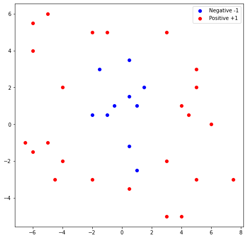
The algorithm we described above finds the linear model that divides the feature space. However, some real-world data is non-linear and a linear model will not be able to effectively classify the data as shown in Figure 5. As shown in the figure, no matter how we try to fit the linear model, the decision boundary will give a bad classification result. One way to deal with this kind of data is to extend the feature dimension by performing data transformation using basis functions such as polynomial and spline [3]. An example of non-linear transformation is given in Figure 5(bottom) whereby the polynomial basis function is used to map the data points from 2-dimension to 3-dimension. After the transformation, we can easily fit a linear model to separate the data points.

We select a basis function, $\phi(\mathbf{x}^i)$ to transform each instance $\mathbf{x}^i$ from $d$ -dimension to $m$ -dimension where $m$ is generally much larger than $d$ . Then, the transformed dataset $\mathbf{\phi}(\mathbf{x}^i) = (\phi_1(\mathbf{x}^i), \phi_2(\mathbf{x}^i), ... \phi_m(\mathbf{x}^i))$ is used to fit the linear model $\hat{f}(\mathbf{\phi}(\mathbf{x}^i)) = \mathbf{w}^T\mathbf{\phi}(\mathbf{x}^i) + b$

Figure 5. Non-linear data and the mapping of the data to a new feature space.

The optimization problem of finding the optimal hyperplane has the same form except the constraints are defined in the new feature space.

$\min \frac{1}{2} \lVert w \rVert^2 + C \sum_{i=1}^N \xi^i$

subject to $y^i(\mathbf{w}^T\mathbf{\phi}(\mathbf{x}^i) + b) - 1 + \xi \geq 0$ and $\xi^i \geq 0$ for $i=1,2,...,N$

Reformulate the problem using Lagrange multiplier.

$L_d = \sum_{i=1}^{N} \lambda^i - \frac{1}{2} \sum_{i=1}^{N} \sum_{j=1}^{N} \lambda^i \lambda^j y^i y^j \mathbf{\phi}(\mathbf{x}^i)^T \mathbf{\phi}(\mathbf{x}^j)$

subject to $\sum_{i=1}^{N} \lambda^i y^i = 0$ and $0 \leq \lambda^i \leq C$ .

Although the mapping of the features to a high dimensional feature space allows the data to be linearly separable, computing the transformation is expensive especially when the dimension is very high. This is because we have to apply the transformation on each sample followed by the inner product. The idea of the kernel trick is that the inner product between the transformed data is not needed. Instead, we require only the kernel function that allows us to operate in the high-dimensional space without computing the data transformation. Therefore, we just need to apply the kernel function, $k$ directly in the original feature space to achieve the same effect.

$k(\mathbf{x}^i, \mathbf{x}^j) = \mathbf{\phi}(\mathbf{x}^i)^T \mathbf{\phi}(\mathbf{x}^j)$

Therefore, $L_d$ is

$L_d = \sum_{i=1}^{N} \lambda^i - \frac{1}{2} \sum_{i=1}^{N} \sum_{j=1}^{N} \lambda^i \lambda^j y^i y^j k(\mathbf{x}^i, \mathbf{x}^j)$

subject to $\sum_{i=1}^{N} \lambda^i y^i = 0$ and $0 \leq \lambda^i \leq C$ . Given the set of support vector indices $S$ , $b$ can be solved

$b^s=y^s - \sum_{m \in S} \lambda^m y^m k(\mathbf{x}^m,\mathbf{x}^s)$

We use an average of all the solutions for numerical stability. Given a test point $\mathbf{\acute{x}}$ , the predicted value is calculate as follows:

$\hat{f}(\mathbf{x}) = \text{sign}( \sum_{s \in S} \lambda^s y^s k(\mathbf{\acute{x}},\mathbf{x}^s) +b)$

Kernels

We discuss some of the commonly used kernel functions in the literature. Polynomial kernel function is defined as

$k(\mathbf{x}, \mathbf{z})=(1+\mathbf{x}^T \mathbf{z})^d$

where $d$ is degree parameter. Consider a dataset with two input features $x_1$ and $x_2$ and a polynomial kernel with a degree of 2.

$\begin{aligned} k(\mathbf{x},\mathbf{z}) & = (1 + \mathbf{x}^T\mathbf{z})^2 \\ & = (1 + x_1 z_1 + x_2 z_2)^2 \\ & = (1 + 2x_1z_1 + 2x_2z_2 + 2x_1x_2z_1z_2 + x_1^2z_1^2 + x_2^2z_2^2) \end{aligned}$

We can see from the above that the dimension of the dataset is extended from 2 to 6.

$\phi(\mathbf{x}) = \begin{bmatrix} 1 \\ \sqrt{2}x_1 \\ \sqrt{2}x_2 \\ 2x_1x_2 \\ x_1^2 \\ x_2^2 \end{bmatrix}$

Radial basis function (RBF) kernel function is similar to the pdf of the normal distribution. The kernel function is defined as

$k(\mathbf{x}, \mathbf{z})=e^{-\gamma \lVert \mathbf{x} - \mathbf{z} \rVert^2}$

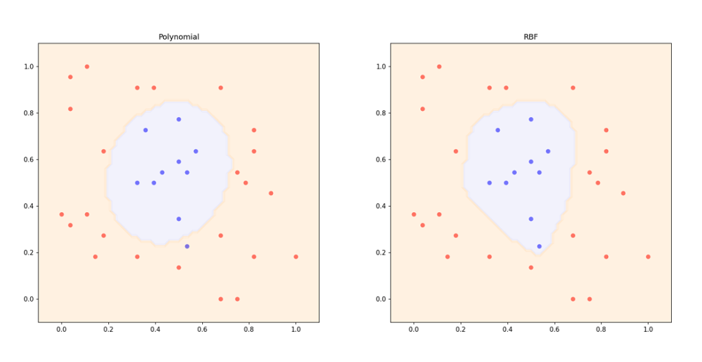
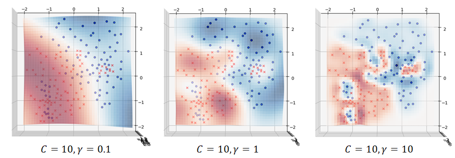
where $\lVert \mathbf{x} - \mathbf{z} \rVert^2$ is the euclidean distance between the two data points and $\gamma$ defines the spread of the kernel or the decision region of the support vectors. In other words, it determines how far the influence of a support vector in the prediction. A small value of $\gamma$ means large decision region area while a large value of $\gamma$ means small decision region area. Figure 6 shows the decision boundaries of non-linear SVM with polynomial and RBF kernels. The effect of $\gamma$ is illustrated in Figure 7.

Figure 6. Decision boundaries of non-linear SVM with polynomial and RBF kernels.

Figure 7. The effect of gamma on the decision boundaries.

Numerical Example

Consider the following dataset. Suppose a non-linear SVM with RBF kernel and $\gamma=0.8$ is built by solving the optimization problem using quadratic programming. The lagrange multipliers $\lambda$ are given as follows.

$\mathbf{x}=\begin{bmatrix} 0.481&0.326\\0.75&0.282\\0.771&0.484\\0.856&0.745\\0.818&0.211\\0.331&0.242 \end{bmatrix}$ $\mathbf{y}=\begin{bmatrix} -1\\-1\\-1\\1\\1\\1\\ \end{bmatrix}$ $\lambda=\begin{bmatrix} 47.777\\37.501\\50.000\\35.278\\50.000\\50.000 \end{bmatrix}$

All data points are support vectors since all $\lambda^i > 0$ . Thus, support vector indices $S={1,2,3,4,5,6}$ . Thus, $b$ can be solved as follows:

$b^s=y^s - \sum_{m \in S} \lambda^m y^m k(\mathbf{x}^m,\mathbf{x}^s)$

$b^1=11.643$ , $b^2=11.370$ , $b^3=15.719$ , $b^4=1.449$ , $b^5=4.832$ , $b^6=-0.683$

$b=\frac{1}{\lvert S \rvert} \sum_{i=1}^{\lvert S \rvert} b^i = 7.388$

Given a test point $\mathbf{\acute{x}}=(0.614,0.258)$ , predict the test point using the SVM model.

$\begin{aligned}\hat{f}(\mathbf{\acute{x}}) &= \text{sign}( \sum_{s \in S} \lambda^s y^s k(\mathbf{\acute{x}},\mathbf{x}^s) +b) \\ &= \text{sign}(-3.717) \\ &= -1 \end{aligned}$

Support Vector Regression

Support vector machine can be generalized for regression problems [4]. Similar to other regression models, support vector regression aims to fit the best line or hyperplane through the data points. However, in support vector regression, the best-fitted hyperplane is not a function that minimizes the error between the real and predicted value. Instead, support vector regression finds a hyperplane such that the margin has the most data points within it while fitting the error to be below a certain threshold $\epsilon$ . In other words, the best-fitted line is the one that has at most $\epsilon$ deviation from the target of the training set.

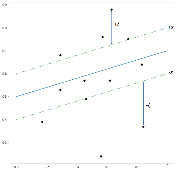
Figure 8 illustrates a support vector regression. The fitted line is indicated by the blue line and the boundary lines of the margin (also known as $\epsilon$ -tube) are indicated by the green dash lines. The error of the data points within the tube is tolerated (zero) while for data points that are outside the tube, the loss is the distance between the data points and the boundary lines. Thus, the loss function is defined as follows.

$L=\begin{cases} 0, & \texttt{if} \lvert y^i - \mathbf{w}^T\mathbf{x}^i + b \rvert < \epsilon \\ \lvert y^i - \mathbf{w}^T\mathbf{x}^i + b \rvert - \epsilon, & \texttt{otherwise} \end{cases}$

Similar to the soft margin hyperplane in support vector classification, the slack variables are introduced to represent the error of data points that are out of the ε-tube. Thus, the optimization problem is given as follows.

$\min \frac{1}{2} \lVert w \rVert^2$

subject to $\begin{cases} \lvert y^i - \mathbf{w}^T\mathbf{x}^i + b \rvert \leq \epsilon + \xi_{+}^i \\ \lvert \mathbf{w}^T\mathbf{x}^i + b - y^i \rvert \leq \epsilon + \xi_{-}^i \\ \xi_{+}^i, \xi_{-}^i \geq 0 \end{cases}$ for $i=1,2,…,N$

Notice that there are two types of slack variables, for positive and negative errors to keep them positive. We restate the optimization problem by applying Lagrange multiplier.

$\begin{aligned} L_p = & \frac{1}{2} \lVert w \rVert^2 + C \sum_{i=1}^N (\xi_{+}^i + \xi_{-}^i) \\ & - \sum_{i=1}^{N} \lambda_{+}^i (\epsilon + \xi_{+}^i - y^i + (\mathbf{w}^T\mathbf{x}^i + b )) \\ & - \sum_{i=1}^{N} \lambda_{-}^i (\epsilon + \xi_{-}^i + y^i - (\mathbf{w}^T\mathbf{x}^i + b )) \\ &- \sum_{i=1}^N \mu_{+}^i \xi_{+}^i - \sum_{i=1}^N \mu_{-}^i \xi_{-}^i \end{aligned}$

$\begin{aligned} L_p = & \frac{1}{2} \lVert w \rVert^2 + C \sum_{i=1}^N (\xi_{+}^i + \xi_{-}^i) \\ & - \sum_{i=1}^N \lambda_{+}^i \epsilon - \sum_{i=1}^N \lambda_{+}^i \xi_{+}^i + \sum_{i=1}^N \lambda_{+}^i y^i - \sum_{i=1}^N \lambda_{+}^i(\mathbf{w}^T\mathbf{x}^i + b) \\ & - \sum_{i=1}^N \lambda_{-}^i \epsilon - \sum_{i=1}^N \lambda_{-}^i \xi_{+}^i - \sum_{i=1}^N \lambda_{-}^i y^i + \sum_{i=1}^N \lambda_{-}^i (\mathbf{w}^T\mathbf{x}^i + b) \\ & - \sum_{i=1}^N \mu_{+}^i \xi_{+}^i - \sum_{i=1}^N \mu_{-}^i \xi_{-}^i \end{aligned}$

Differentiate $L_p$ with respect to $w$ , $b$ and $\xi$ , and set it to zero.

$\frac{\partial L_p}{\partial w}=0$ , $w=\sum_{i=1}^{N} (\lambda_{+}^i - \lambda_{-}^i ) \mathbf{x}^i$

$\frac{\partial L_p}{\partial b}=0$ , $\sum_{i=1}^{N} (\lambda_{-}^i - \lambda_{+}^i) = 0$

$\frac{\partial L_p}{\partial \xi_{+}}=0$ , $C - \sum_{i=1}^{N} (\lambda_{+}^i + \mu_{+}^i) = 0$

Substitute the derivatives into $L_p$ and simplify it.

$\begin{aligned} L_p = & \frac{1}{2} \sum_{i=1}^N \sum_{j=1}^N (\mathbf{x}^i)^T \mathbf{x}^j (\lambda_{+}^i - \lambda_{-}^i)(\lambda_{+}^j - \lambda_{-}^j) + \sum_{i=1}^N (\lambda_{+}^i + \mu_{+}^i) \sum_{i=1}^N (\xi_{+}^i + \xi_{-}^i) \\ & + \sum_{i=1}^N y^i(\lambda_{+}^i - \lambda_{-}^i) - \sum_{i=1}^N \epsilon (\lambda_{+}^i + \lambda_{-}^i) \\ & - \sum_{i=1}^N \lambda_{+}^i \xi_{+}^i - \sum_{i=1}^N \lambda_{-}^i \xi_{-}^i - \sum_{i=1}^N \mu_{+}^i \xi_{+}^i - \sum_{i=1}^N \mu_{-}^i \xi_{-}^i \end{aligned}$

$\begin{aligned} L_p = & \frac{1}{2} \sum_{i=1}^N \sum_{j=1}^N (\mathbf{x}^i)^T \mathbf{x}^j (\lambda_{+}^i - \lambda_{-}^i)(\lambda_{+}^j - \lambda_{-}^j) \\ & + \sum_{i=1}^N y^i(\lambda_{+}^i - \lambda_{-}^i) - \sum_{i=1}^N \epsilon (\lambda_{+}^i + \lambda_{-}^i) \\ & + \sum_{i=1}^N \lambda_{+}^i \xi_{+}^i + \sum_{i=1}^N \lambda_{+}^i \xi_{-}^i + \sum_{i=1}^N \mu_{+}^i \xi_{+}^i + \sum_{i=1}^N \mu_{+}^i \xi_{-}^i \\ & - \sum_{i=1}^N \lambda_{+}^i \xi_{+}^i - \sum_{i=1}^N \lambda_{-}^i \xi_{-}^i - \sum_{i=1}^N \mu_{+}^i \xi_{+}^i - \sum_{i=1}^N \mu_{-}^i \xi_{-}^i \end{aligned}$

subject to $\begin{cases} \sum_{i=1}^{N} (\lambda_{-}^i - \lambda_{+}^i) = 0 \\ 0 \leq \lambda_{+}^i \leq C \\ 0 \leq \lambda_{-}^i \leq C \end{cases}$ .

Upon solving the optimization problem using quadratic programming, data points that lie within $\epsilon$ -tube have $\lambda_{+}^i = \lambda_{-}^i = 0$ . The support vectors have $\lambda_{+}^i > 0$ or $\lambda_{-}^i>0$ , and we use them to calculate $b$ . The dot product $(\mathbf{x}^i)^T \mathbf{x}^j$ can be replaced with a kernel $k(\mathbf{x}^i, \mathbf{x}^j)$ and we can have a non-linear support vector regression.

References

[1] J. Nocedal and S. J. Wright, Numerical optimization. Springer, 1999.

[2] C. Cortes and V. Vapnik, “Support-vector networks,” Mach Learn, vol. 20, no. 3, pp. 273–297, Sep. 1995, doi: 10.1007/BF00994018.

[3] B. E. Boser, I. M. Guyon, and V. N. Vapnik, “A training algorithm for optimal margin classifiers,” in Proceedings of the fifth annual workshop on Computational learning theory, New York, NY, USA, Jul. 1992, pp. 144–152. doi: 10.1145/130385.130401.

[4] H. Drucker, C. J. Burges, L. Kaufman, A. Smola, and V. Vapnik, “Support vector regression machines,” Advances in neural information processing systems, vol. 9, 1996.