Convolutional Neural Network

Introduction

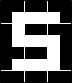
Unstructured data such as images and time series contain rich information both in spatial and temporal domains. Take image data as an example, the spatial structure of the pixels defines the visual information of the data. Figure 1 illustrates an image with 7 rows and 6 columns of pixels. The black and white pixels are arranged to form a digit of 5.

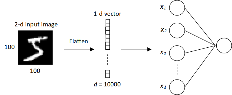
Figure 1. An image with 7 rows and 6 columns of black and white pixels.

As has been described in Supervised Learning section, to predict image data using machine learning algorithms, the 2-d input is transformed into a 1-d feature vector consisting of the pixel values. Specifically, a single pixel represents an input to the predictive model, which means the number of inputs is equal to the number of pixels. Although this approach seems feasible, the input data is noisy and high-dimensional, and increase the model complexity. For example, in a fully-connected neural network, each unit in a layer is connected to each unit in the subsequent layer. By defining using such a neural network, the number of weights will be tremendously high because we need a different weight for every single neural connection. Consider a black and white image of $100 \times 100$ being classified by a neural network as shown in Figure 2. The 2-d image data is flattened into a feature vector of size 10000. If there are 10000 units in the hidden layer, there will be 100 million neural connections between the input and hidden layers whereby each connection is having different weight parameter. Furthermore, since the 2-d input data is flattened into a 1-d vector, all spatial information is completely lost and cannot be leveraged by the neural network.

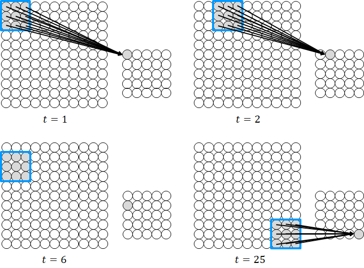
Figure 2. The spatial information is lost due to flattening and the number of input units of the neural network is equal to the number of pixels.

As we mentioned above, image data has rich spatial information which could be used in the prediction task. How do we leverage this information in the neural network? To leverage the spatial information, instead of taking all the pixels for processing, we define a small region of the image and process the pixels in that region. Consider an image as a 2-d array of pixel values where each pixel value is an input unit of the neural network as shown in Figure 3. A small region or called filter is defined, in this case, $3 \times 3$ pixels as indicated by the blue square. We connect the input pixels in the region to a single unit of the hidden layer. Similarly, each connection has a weight that defines the strength of the connection. Thus, essentially, the filter is a set of weights that are learned using the backpropagation algorithm.

We define the same neural connections across the whole input pixels as shown in the figure. To do this, the window is slid across the whole input image from the left edge to the right edge, followed by sliding the window downward until it reaches the bottom right corner of the image. In this way, the units of the hidden layer only see a particular region of the image which allows the network to extract features or details from the spatially closed pixels. Furthermore, the number of weights is reduced significantly since the units of the hidden layer are connected to only a fraction of the input pixels. Also, since the weights are shared across the input image, features that matter in one part of the image can be extracted by the filter in another part of the image. This filter operation is called convolution.

Figure 3. Patches of input pixels are connected to the units of the hidden layer.

Feature Extraction and Convolution

Figure 4 demonstrates the motivation of feature extraction and how the features can be extracted by the convolution operation. The figure shows two images of a digit of five. The image on the right contains noises, hence the digit is a bit distorted or deformed. If we are to classify the image by performing a pixel-by-pixel comparison, the right image will be misclassified. A better way to classify the images is to identify the features of a digit of five. A feature is a specific part of the image with a certain pattern that characterizes a particular object, which can be used to identify an object. For example, the features of a digit of five are indicated by the red boxes. Feature 1 and feature 2 characterize the corners while feature 3 characterizes the horizontal line of the digit. If these features can be detected on the deformed image roughly at the same location, we can conclude that the image is indeed a digit of five.

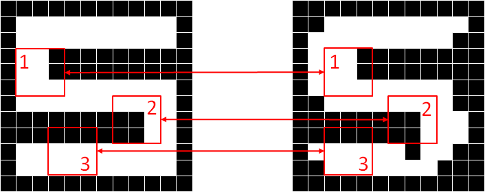
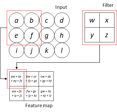
Figure 4. The features of the image are indicated by the red regions.

Figure 5 illustrates an example of applying convolution on a 2-d input image. Convolution operation involves applying element-wise multiplication between the values of the filter and the pixel values of the small region, followed by taking the summation of the multiplications. As shown in the figure, the red boxes indicates the first convolution operation involving the filter and the region containing pixel a, b, e and f. The convolution operation on the input image produces an output of $2 \times 3$ . The output of the convolution is known as feature map.

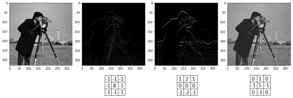
Figure 5. Convolution operation involving a filter of 2 x 2 and an image of 3 x 4. The output of the feature map indicated by the red box is produced by the applying the filter to the corresponding top left region of the input image.

The feature map indicates wherein the input image, the feature has been detected by the filter i.e. high values of the feature map represent greater activation or detected features. By simply changing the weights of the filter, different feature maps can be produced as shown in Figure 6. As can be seen in the figure, three different filters have been applied to the original image on the left generating three different outputs.

Figure 6. The original image on the left is applied with three different filters. The first two images are applied with two different edge detection filters and the last image is sharpened with the sharpen filter.

Convolutional Neural Network

We have seen how convolution operation capitalizes spatial structure that is inherent in image data to detect and extract local features. This concept of preserving the spatial structure and feature extraction is at the core of convolutional neural networks (CNN). A convolutional neural network minimally consists of a convolutional layer, a pooling layer and a fully connected layer [2]. The convolutional layer aims to extract discriminative local features directly from the image data. To extract the optimal features for the prediction, the weights of the filters are optimized during the backpropagation phase.

The purpose of the pooling layer is to downsample the size of the feature map to reduce the computational cost. Furthermore, a pooling layer suppresses the irrelevant information in the feature map to improve the performance of the prediction. We will discuss pooling layers in the following section. Lastly, the fully-connected layer is the traditional neural network layer where each unit is connected to the units of the subsequent layer. The multi-dimensional feature maps are flattened into a 1-d feature vector which will be used as the input layer to the fully-connected layer(s) for classification or regression.

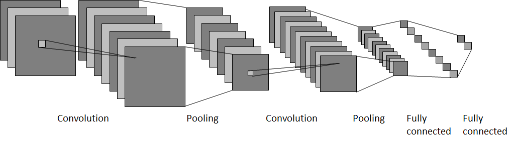
Typically, a CNN has a series of alternating convolutional and pooling layers before the fully-connected layers. The subsequent convolutional and pooling layers take the feature map previously generated by the convolutional and pooling layer as input and perform convolution operations to produce a feature map which in turn is reduced by the pooling operations. This allows the network to learn the features in a hierarchical manner, producing more salient features [1]. Figure 7 illustrates an example of a convolutional neural network consisting of two convolutional layers and two pooling layers in between, followed by two fully-connected layers.

Figure 7. A convolutional neural network consists of convolutional, pooling and fully-connected layers.

Convolutional Layer

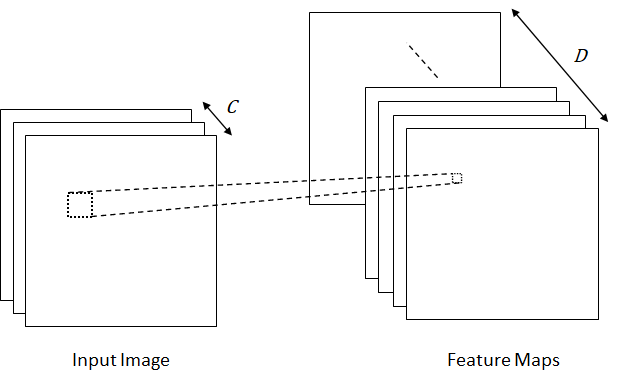
A convolutional neural network consists of convolutional, pooling and fully-connected layers. Let $l$ be the $l$ -th layer where $l=1$ is the first layer and $L$ is the last layer. A convolutional layer consists of a set of different filters to extract different types of features as shown in Figure 8. Let $K \in \mathbb{R}^{k_1 \times k_2 \times C \times D}$ denotes the set of filters where $k_1$ and $k_2$ represent the height and width of the filters, $C$ is the number of input channels and $D$ is the number of filters or the depth of the feature maps (number of feature maps).

Given an input image with $C=1$ channel (grayscale image) and a filter $w$ of size $k_1 \times k_2$ , the convolution operation produces feature map $d$ as follows:

$z_{i,j,d}^{(l+1)} = \sum_{m=1}^{k_1} \sum_{n=1}^{k_2} w_{m,n,d}^{(l)} \cdot a_{i+m,j+n}^{(l)} + b$

$a_{i,j,d}^{(l+1)} = g(z_{i,j,d}^{(l+1)})$

where $b$ is the bias, $z_{i,j,d}$ is the output of feature map $d$ with $i$ -th row and $j$ -th column, $g$ is an activation function applied to each output of the feature map.

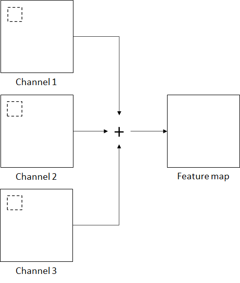
In the case of color images with $C=3$ channels, each channel has a filter of the same size but with different set of weights as shown in Figure 9. The convolution operation is applied independently to each of the channels, yielding three sets of outputs which are summed to produce a single feature map. The convolution operation is defined as follows:

$z_{i,j,d}^{(l+1)} = \sum_{m=1}^{k_1} \sum_{n=1}^{k_2} \sum_{c=1}^C w_{m,n,c,d}^{(l)} \cdot a_{i+m,j+n,c}^{(l)} + b$

Figure 9. Applying convolution on multi-channel input produces a feature map.

Based on the above definition, the size of the feature maps is determined by the filter size. Another parameter that affects the size of the feature map is the stride which is the number of pixels that the filter is shifted (slid) over the input along the width and height. Typically, the stride is set to 1. However, we can set stride to a larger value which results in a feature map with a smaller size. Consider an input image of $9 \times 9$ is convolved with a filter of $3 \times 3$ as shown in Figure 10. The convolution operation with a stride value equal to 1 produces a feature map of $7 \times 7$ and a feature map of $4 \times 4$ is produced when the stride is equal to 2.

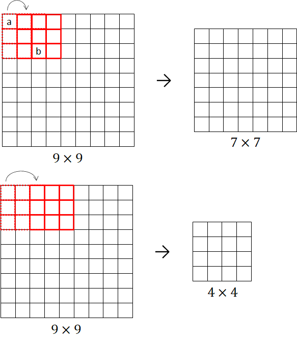
Figure 10. Convolution with stride equal to 1 and 2, producing feature maps of 7 x 7 and 4 x 4 respectively.

We see that applying convolution operation with $3 \times 3$ filter and stride equals 1 to the $9 \times 9$ input image results in a feature map with the size of $7 \times 7$ , a reduction of about 40% of the total input pixels. The sliding window from the top left corner to the bottom right corner results in not only a reduced feature map but also the corner and edge pixels of the input image having a minimal contribution to the output of the convolution operation. This is because the pixels are processed much less than those in the middle. As shown in Figure 10(top), pixel ‘a’ is used only in one convolution operation while pixel ‘b’ is used in nine convolution operations. Evidently, the information at the edges is not preserved as well as the information in the middle of the input image.

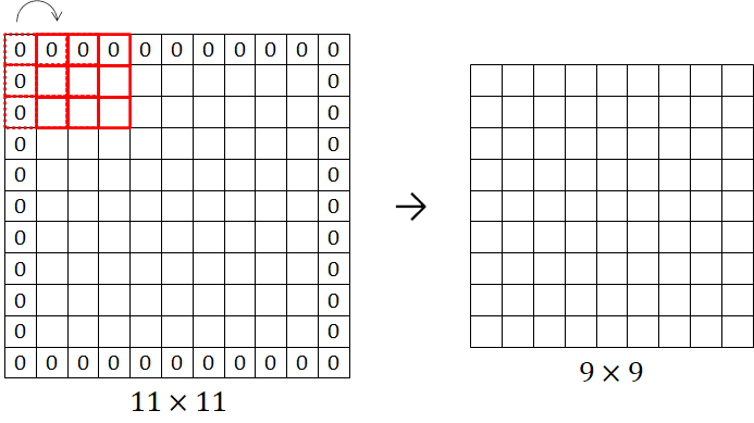
A solution to the problem is to pad the input image with extra zero pixels around its boundary. The padding allows the corner and edge pixels to be the middle pixels, thus increasing their contribution to the output of the convolution operation and consequently preserving the information at the edges of the input image. Furthermore, it produces a feature map with the same size as the input image (before the zero padding). Consider a $9 \times 9$ input image is padded with zero pixels as shown in Figure 11. As shown in the figure, there is one-pixel border which means the amount of zero padding is one. A filter of $3 \times 3$ with a stride equal to 1 is applied to the input image resulting in a feature map with a size of $9 \times 9$ .

Figure 11. The boundary of the input image is padded with extra zero pixels.

Pooling Layer

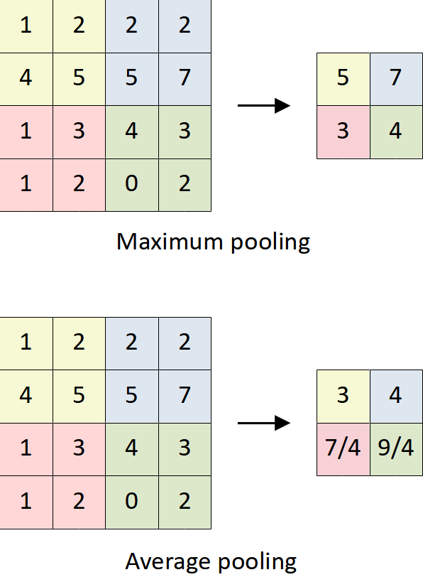
While the role of a convolutional layer is to extract features from the input data, the role of a pooling layer is to reduce the size of the feature maps by mapping patches of activations to a single activation value. The pooling operation works by defining a window that is similar to a filter and applying it to the feature map along both width and height. For each window, the pooling operation summarizes the presence of the feature values in the window. There are pooling operations which are computing the maximum values and averaging the values in the window. The maximum pooling returns the most prominent activation while the average pooling returns the average of the activations in the window. In general, maximum pooling (or max-pooling) is the most commonly used in convolutional neural networks.

Typically, the window size or pool size is $2 \times 2$ with a stride equals 2 which means the window is not overlapping when it is slid from left to right and from top to bottom, reducing 75% of the activations of the feature map. Unlike convolutional layers, pooling layers operate independently on every slice of the feature maps which means a convolutional layer only spatially resizes while keeping the depth of the feature maps. Figure 12 shows a $4 \times 4$ feature map is reduced with a pool size of $2 \times 2$ and a stride of 2 using maximum and average pooling operations, producing a $2 \times 2$ feature map.

The use of pooling layers has several advantages. First, the dimension of the feature representation can be reduced, consequently reducing the computation time and the weights of the neural network. Secondly, a feature map contains the detected features and their positions in the input image. A slight change to the positions of the features in the input image results in a different feature map. Pooling layers discard the positions of the detected features and keep only the prominent features, thereby producing translation invariance features that are more robust and reliable [3]. In convolutional neural networks, the convolutional layer and pooling layer are stacked alternately to extract and downsample features in a hierarchical manner. However, in a very deep neural network, the number of pooling layers is relatively lesser than the number of convolutional layers because the pooling operation can drastically reduce the size of the feature map. Thus, fewer pooling layers are required to reduce the feature map to the desired size.

Figure 12. Maximum pooling returns the maximum activations while average pooling returns the average of the activations in the window.

Fully Connected Layer

In a convolutional neural network, the series of convolutional and pooling layers is known as feature learning pipeline, which is used to learn the feature representation. The feature learning pipeline is followed by a series of fully connected layers for prediction. Typically, the last feature maps that are produced by the feature learning pipeline are flattened to a 1-d feature vector. The feature vector is then used as input to the fully connected layers by connecting each feature (activation) to each unit of the first hidden layer. These fully connected layers works exactly the same way as the traditional neural networks. One might apply the ReLU, sigmoid or tanh after each hidden layer. As for the output layer, the number of units and activation function depends on the specific requirements of the application. It is noteworthy that the fully connected layers are densely connected, thus the majority of the weights of the network lie in these layers. Although there is no recommended size for the last feature maps, one might want to go as low as possible to reduce the overall number of weights.

References

[1] Y. LeCun, Y. Bengio, and G. Hinton, “Deep learning,” Nature, vol. 521, no. 7553, Art. no. 7553, May 2015, doi: 10.1038/nature14539.

[2] S. Skansi, Introduction to Deep Learning: from logical calculus to artificial intelligence. Springer, 2018.

[3] I. Goodfellow, Y. Bengio, and A. Courville, “Deep learning (adaptive computation and machine learning series),” Cambridge Massachusetts, pp. 321–359, 2017.