Artificial Neural Network

Artificial Neural Network or simply Neural Network (ANN) is a machine learning technique that is modeled loosely after the human brain. It is a powerful, scalable and versatile technique that has been used to solve highly complex problems such as e-mail spam filtering, machine translation and pattern recognition (see how convolutional neural networks (deep learning) can be used to automatically extract features from data). The fundamental building block of a neural network is the perceptron. Recall that a perceptron is a hyperplane that divides the feature space into positive and negative regions. The prediction of the hyperplane is defined by

$\hat{f}(\mathbf{x}) = \text{sign} (\sum_{j=0}^d w_jx_j)=\mathbf{w}^T\mathbf{x}$

where $\mathbf{x}$ is the feature vector and $\mathbf{w}$ is the weight vector that defines the hyperplane. This computation can be represented by a network diagram as shown in Figure 1.

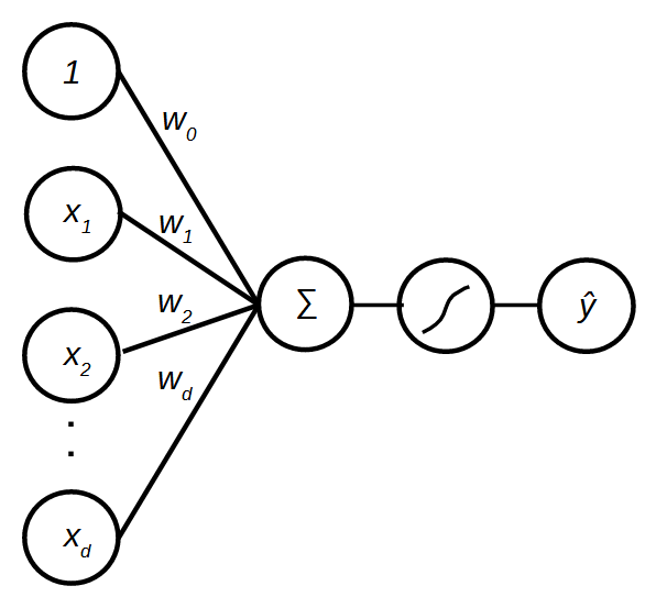
Figure 1. A network diagram of perceptron.

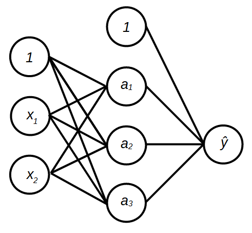
The perceptron accepts an arbitrary number of inputs features $x_j$ , and each input is associated with a weight $w_j$ . The linear combination of the inputs is then fed to the sign function to produce the prediction $\hat{y}$ . Multiple perceptrons can be stacked on top of each other, forming a layer of output, and this layer of perceptrons can be connected to another layer of perceptrons as shown in Figure 2. This model is known as multilayer perceptron aka neural network. Note that an individual perceptron (later referred to as a unit) is simplified by representing the summation, sign function and prediction with a single node $a_j$ . As can be seen in the figure, the neural network has two layers of units, an intermediate layer (also known as a hidden layer) and an output layer. Thus, we have two sets of weights, one is for the hidden layer and the second set is for the output layer. The output layer is not directly connected to the input features. Instead, the output layer gets its inputs from the hidden layer which maps the inputs to a new feature space. We can think of this as deriving a new set of inputs for the prediction.

Figure 2. Multilayer of perceptrons or known as neural network.

In neural network, the sigmoid function is used instead of the sign function. The sigmoid function which is also known as activation function is used to introduce non-linearity to the model. This will help the neural network to learn non-linear decision boundaries.

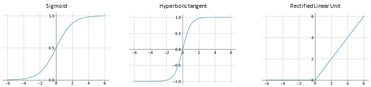
Sigmoid function maps the input to any value range between $(0,1)$ as shown in Figure 2(left). It has a nice property where it tends to bring the activations towards 0 or 1 due to the steep slope in the middle of the function. However, the gradient at either tail of 0 or 1 is very small or almost zero. This may cause the weights of the network are not to be updated during training. This problem is known as vanishing gradient. Sigmoid function is defined as follows:

$\mathbf{a}(\mathbf{z}) = \frac{1}{1+e^{-\mathbf{z}}}$

where $\mathbf{z}=\mathbf{w}^T\mathbf{x}$ is the inner product between the weight vector $\mathbf{w}$ and the input vector $\mathbf{x}$ .

Besides sigmoid function, the commonly used activations are hyperbolic tangent (tanh) and rectified linear unit (ReLU). Tanh is similar to sigmoid function. Instead of mapping the input to any value in the range of $(0,1)$ , the output of the function is in the range of $(-1,1)$ . This is shown in Figure 2(middle) It is closely related to sigmoid because the following holds.

$\mathbf{a}(\mathbf{z})=2\sigma(2\mathbf{z})-1$

where $\sigma$ is the sigmoid function. Although they have similar properties, tanh is preferred because it often converges faster than the sigmoid [1].

ReLU is a piecewise linear function whereby it is linear for all positive values and zero for all negative values as shown in Figure 3. Compared to sigmoid and tanh, ReLU is simpler to compute and therefore take less time to train and execute. Unlike sigmoid and tanh, ReLU does not suffer from saturation or vanishing gradient. However, ReLU may cause some units to always output zero due to the zero gradient at $z \leq 0$ . As a result, the units are not taking part in the prediction [2]. ReLU function is defined as follows:

$\mathbf{a}(\mathbf{z})=\max(0,\mathbf{z})$

Various variant of ReLU have been proposed such as Leaky ReLU and exponential liner unit (ELU).

Figure 3. The commonly used activation functions.

Forward Propagation

The output of the neural network is obtained by propagating the inputs through the hidden layer to the output layer. Let $L$ is the number of layers in a neural network. Hence, in this example $L=3$ where $l=1$ is the input layer and $l=2$ is the hidden layer. The weights including the bias are denoted by $\mathbf{w}$ where $w_{ij}^{(l)}$ denote the weight associated with the connection between unit $j$ in layer $l$ and unit $i$ in layer $l+1$ . The $w_{i0}^{(l)}$ is the bias associated with unit $i$ in layer $l+1$ . We denote the $j$ -th input as $x_j$ . The forward propagation of input $x_j$ to the units of the next layer is given as follows.

$z_1^{(2)}= w_{10}^{(1)} + w_{11}^{(1)}x_1 + w_{12}^{(1)}x_2$

$z_2^{(2)}= w_{20}^{(1)} + w_{21}^{(1)}x_1 + w_{22}^{(1)}x_2$

$z_3^{(2)}= w_{30}^{(1)} + w_{31}^{(1)}x_1 + w_{32}^{(1)}x_2$

$a_1^{(2)}= g(z_1^{(2)})$

$a_2^{(2)}= g(z_2^{(2)})$

$a_3^{(2)}= g(z_3^{(2)})$

where $g(z_j^{(l)})$ is the activation function. The propagation of the signals to the output layer follows the same computation.

$z^{(3)}=w_{0}^{(2)} + w_1^{(2)}a_1^{(2)} + w_2^{(2)}a_2^{(2)} + w_3^{(2)}a_3^{(2)}$

$\hat{y} = a^{(3)} = g(z^{(3)})$

We can generalize the forward propagation as follows:

$z_i^{(l+1)} = \sum_{j=0}^{s_l} w_{ij}^{(l)} a_i^{(l)}$

$a_i^{(l+1)} = g(z_i^{(l+1)})$

where $s_l$ is the number of units in layer $l$ .

Output Layer

Neural networks can be used for both classification and regression. For regression, the number of units is equal to the number of output responses. For example, if there are three responses, the number of units at the output layer is three. The activation function is typically linear $\mathbf{a}(\mathbf{x}) = z(\mathbf{x})$ . ReLU or sigmoid function is used if the response is normalized.

For binary classification, one unit is sufficient at the output layer to represent both classes. The sigmoid function is used to obtain an output value in the range of $(0,1)$ . This is similar to logistic regression. If the predicted value is above 0.5, assign the test input to class 1. Otherwise, assign it to class 0.

For multiclass classification, the number of units is equal to the number of classes. The $c$ th unit represents the probability of class $c$ whereby the sum of the probabilistic outputs is 1. Softmax function is used to ensure the output is probabilistic.

$\hat{y}_j = \frac{e^{z_j}}{\sum_{c=1}^C e^{z_c}}$

Backward Propagation Algorithm

The weights of the neural networks need to be estimated to solve the prediction problem. The estimation of the weights (also known as training or learning) is a process of finding the weight and bias values that will produce the desired output at the output layer when a certain input is given to the network. How does a neural network learn? For a human to learn to do things, we will be told whether we are doing it right or wrong. For example, if we are to learn to play football, we watch how the ball flies as we kick the ball. The next time we kick the ball, we remember the mistake that we have done before and improvise the movement to kick the ball a bit better. Similarly, a neural network learns to solve a problem by comparing the output that is produced by the network with the output that was meant to produce. The difference between the neural network’s output and the label (true output) is the amount of error that the neural network needs to reduce to improve its prediction. The error is calculated using the loss function. The choice of the loss function depends of the prediction problem. For regression problem, the mean squared error is used while the negative log-likelihood (cross entropy) is used for classification problem.

$J_{sq}(\hat{f})=\frac{1}{N} \sum_{i=1}^{N} (y^i-\hat{f}(\mathbf{x})^i)^2$

$J_{nll}(\hat{f}) = -\frac{1}{N} \sum_{i=1}^N \sum_{c=1}^C y_c^i \log_e{\hat{f}_c(\mathbf{x}^i)}$

$J(\hat{f})$ is a measure of how badly the network is performing. Thus, the loss function needs to be minimized in order for the neural network to produce the correct output.

Minimizing the loss function involves adjusting the weights of the connections between two units in the network. The weights are adjusted in such a way that the output that will be produced by the network is close to the actual output. This involves propagating the error from the output layer to the hidden layer(s). Hence the process is known as backward propagation (or backpropagation). The backpropagation is performed using the gradient descent.

The backpropagation algorithm computes the partial derivatives (gradients) of the loss function with respect to each weight of the neural network. Consider the neural network in Figure 2.

The gradient with respect to the weights connecting the hidden layer to the output layer is

$\frac{\partial J}{\partial w_{ij}^{(2)}} = \frac{\partial J}{\partial \hat{y}} \cdot \frac{\partial \hat{y}}{\partial z_{ij}^{(2)}} \cdot \frac{\partial z_{ij}^{(2)}}{\partial w_{ij}^{(2)}}$

The gradient with respect to the weights connecting the input layer to the hidden layer is

$\frac{\partial J}{\partial w_{ij}^{(1)}} = \frac{\partial J}{\partial \hat{y}} \cdot \frac{\partial \hat{y}}{\partial z_{ij}^{(2)}} \cdot \frac{\partial z_{ij}^{(2)}}{\partial a_{ij}^{(1)}} \cdot \frac{\partial a_{ij}^{(1)}}{\partial z_{ij}^{(1)}} \cdot \frac{\partial z_{ij}^{(1)}}{\partial w_{ij}^{(1)}}$

Then, the weights are updated using the computed gradients.
$w_{ij}^{(l)} := w_{ij}^{(l)} - \alpha \frac{\partial J}{\partial w_{ij}^{(l)}}$

where $\alpha$ is the step size or learning rate. Note that $:=$ is an assignment operator.

Variants of Gradient Descent

There are three variants of gradient descent for training neural networks. The variants are batch gradient descent, stochastic gradient descent and mini-batch gradient descent.

Batch Gradient Descent

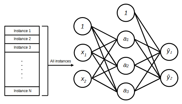
In batch gradient descent, all the training instances are fed to the network, the error for each training instance is calculated and the average is taken over all the errors. The average error is then used to update the weights of the neural network. Since the error is calculated over all training instances, the gradient is a good estimate of the true gradient and the training is stable. Also, the computation is less demanding since the weights are updated only once per epoch. However, the training could get stuck at the saddle point or suboptimal minimum because the calculated gradient is the same for every weight update.

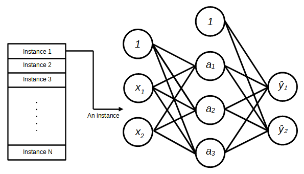
Figure 4. The whole training set is fed to the network to update the weights.

Stochastic Gradient Descent

In stochastic gradient descent, instead of the whole training set, a single training instance is used to calculate the error and update the weights. Since the gradient is estimated on a single instance, the gradient is noisy and it is more difficult to find the optimal minimum. Thus, it will take longer to train the model. Also, stochastic gradient descent is computationally intensive due to the frequent weight update. However, due to the noisy gradient, training may escape saddle point and suboptimal minimum.

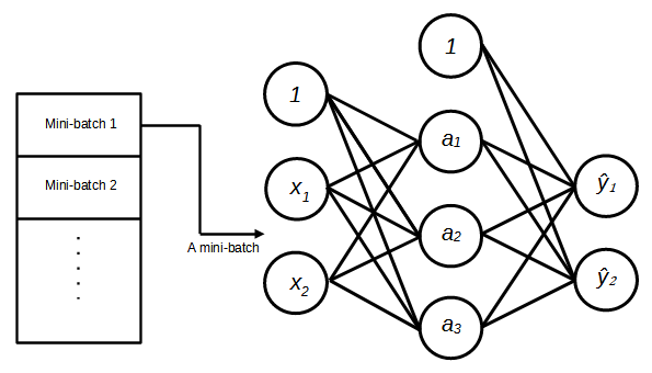
Figure 5. One instance is fed to the network at a time to update the weights.

Mini-batch Gradient Descent

Mini-batch gradient descent is the commonly used technique for training neural networks. In mini-batch gradient descent, the training set is split into a number of small batches. During training, one batch is fed to the network at a time, the error is calculated over that mini-batch and used to update the weights. The gradient is less noisy compared to stochastic gradient descent. Thus, the training is more stable and easier to find the optimal minimum and is more computationally efficient.

Figure 6. A mini-batch is fed to the network at a time to update the weights.

References

[1] Y. A. LeCun, L. Bottou, G. B. Orr, and K.-R. Müller, “Efficient BackProp,” in Neural Networks: Tricks of the Trade: Second Edition, G. Montavon, G. B. Orr, and K.-R. Müller, Eds. Berlin, Heidelberg: Springer, 2012, pp. 9–48. doi: 10.1007/978-3-642-35289-8_3.

[2] L. Lu, Y. Shin, Y. Su, and G. E. Karniadakis, “Dying ReLU and Initialization: Theory and Numerical Examples,” CiCP, vol. 28, no. 5, pp. 1671–1706, Jun. 2020, doi: 10.4208/cicp.OA-2020-0165.

[3] D. E. Rumelhart, G. E. Hinton, and R. J. Williams, “Learning representations by back-propagating errors,” Nature, vol. 323, no. 6088, Art. no. 6088, Oct. 1986, doi: 10.1038/323533a0.