Introduction
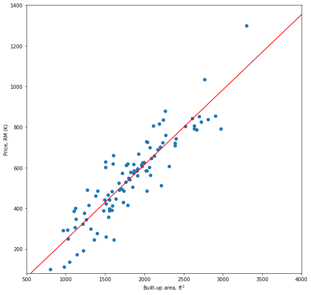
A regression problem is when the response variable is continuous,  such as salary, height, price etc. Consider a regression problem of predicting the price of a house given its built-up area. The data is given in Figure 1. The built-up area is the input feature,
  and the price is the response variable,
  which can take values ranging from RM100,000 to RM1,300,000.
Linear regression is one of the most widely used algorithms for solving regression problems. The algorithm assumes the response has a linear relationship with the input feature. Thus, the linear regression model is expressed as

where  is the intercept and
  is the inner product between the model’s parameters (or weights) and the input features.
Suppose the input is 1 dimensional (there is only one feature as above), the linear regression model is represented as follows:

where the and  are the intercept and the slope respectively. This is known as univariate (simple) linear regression. A univariate linear regression model is fitted to those data points. The fitted line is indicated by the red line.
The univariate linear regression can be generalized to multivariate linear regression where the input is  dimensional data points. Consider the problem of predicting house price, in addition to the built-up area, the inputs can be the number of rooms, the number of floors, location etc. The model is known as multivariate linear regression. A common notational trick is to introduce a constant input,
  whose value is always 1. Thus, the intercept term can be combined with the other terms as follows:

Model Parameters
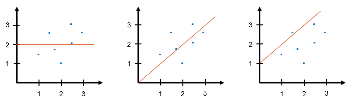
The role of weights is to define the direction of the fitted line. Let’s review the role of intercept and slope in univariate linear regression. Figure 2 illustrates three linear models with different parameters.
Linear model 1, on the left of the figure, the weights are  ,
,  . Since the slope is 0 and the intercept is 2, the linear model is a horizontal line crossing 2 at the y-axis.
Linear model 2, in the middle of the figure, the weights are  ,
,  . The slope of the model is 1 and the intercept is 0. Hence the linear model has an upward trend, and the line is going through the origin.
Finally, linear model 3, on the right of the figure, the weights are  , . The linear model has a similar trend with linear model 2. However, the line is crossing 1 at the y-axis due to its intercept being 1.
Now, how do we find the parameters that will give us an optimal linear regression model? Essentially, the idea is we want to choose weights such that the linear regression model will give us prediction  that is close to the response, . This is formulated by choosing a set of weights,
  that minimizes the sum of squared loss (the difference between the response and the predicted value) over all the training instances. We ignore the fraction
  to simplify the explanation. Ignoring the fraction will not affect the parameter estimation since it is a constant.

Least Squares
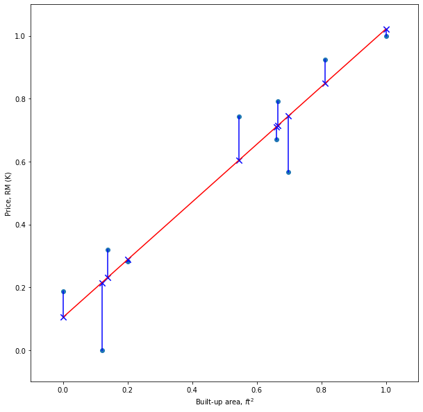
The common method to estimate the weights that will minimize the loss function is the least squares. The method is illustrated in Figure 3. The data points are indicated by the blue dots and the red line is the linear regression model. The predicted value for each training instance is shown as blue crosses. The blue line from a data point to the blue cross is the prediction error which is the difference between the response and the predicted value. The aim is to find a set of weights that will minimize the sum of squared errors.
Let’s express the loss function using matrix notation.

Differentiating  with respect to .

Set the derivative to zero to solve for .


The optimal weights of the linear regression model is given by

It might happen that the least squares fail to provide the optimal weights. This occurs when the input features are (perfectly) correlated e.g.  . Then, the
  is singular (determinant is zero) and the inverse of the matrix does not exist.
Numerical Example
Given the following dataset, find using least square and gradient descent.


Calculate 


Gradient Descent
The weights of the linear regression model can be estimated using an optimization algorithm known as gradient descent. Gradient descent is an algorithm for finding a local minimum of a differentiable function. Note that, gradient descent is a generic algorithm that is used not only in linear regression but it is applied in various places in machine learning. In the context of linear regression, the squared loss is a differentiable function, thus gradient descent can be used to find the weights that will minimize the loss function. Unlike least squares, gradient descent solves the optimization problem in an iterative manner. The weights are iteratively updated based on the derivative of the loss function. For iterative  , the weights are updated as follows:

where  is the learning rate which control the amount of update to be applied to the weights,
  is the derivative of the loss function with respect to each weight,
  which can be written as follows:


 is a mathematical convenience to cancel out 2 when derivative is performed on the loss function.
Numerical Example
Given the following dataset, find using least square and gradient descent.
Randomly initialize .

Calculate 

Calculate the loss using mean squared error.

Calculate the gradient with respect to


Suppose  . Update .


Using the updated , calculate (new) prediction and loss.

Notice that the loss is decreased after the weight update. The steps are repeated until the error is converged.